Batch Effect Correction in Genomic Data: A Comprehensive Guide for Robust Biomedical Research
This article provides a comprehensive guide for researchers and drug development professionals on addressing the pervasive challenge of batch effects in genomic data analysis.
Batch Effect Correction in Genomic Data: A Comprehensive Guide for Robust Biomedical Research
Abstract
This article provides a comprehensive guide for researchers and drug development professionals on addressing the pervasive challenge of batch effects in genomic data analysis. It covers foundational concepts, explores method-specific correction strategies for diverse data types including RNA-seq, single-cell, DNA methylation, and proteomics, discusses troubleshooting and optimization techniques, and delivers a comparative analysis of leading correction tools. By synthesizing the latest methodologies and validation frameworks, this guide aims to empower scientists to enhance data reliability, improve reproducibility, and ensure the biological validity of their genomic findings.
What Are Batch Effects? Diagnosing Technical Noise in Your Genomic Datasets
FAQs on Batch Effects
1. What is a batch effect? A batch effect is a form of non-biological variation introduced into high-throughput data due to technical differences when samples are processed and measured in separate groups or "batches." These variations are unrelated to the biological question under investigation but can systematically alter the measurements, potentially leading to inaccurate conclusions [1] [2].
2. What are the most common causes of batch effects? Batch effects can arise at virtually every stage of an experiment. Key sources include [1] [2]:
- Reagent Lots: Using different batches or lots of chemicals and kits.
- Personnel: Differences in technique between individual researchers.
- Instrumentation: Using different machines or sequencers for measurement.
- Laboratory Conditions: Fluctuations in temperature, humidity, or other environmental factors.
- Time: Conducting experiments on different days or over extended periods.
- Protocols: Variations in sample preparation, storage, or analysis pipelines.
3. Why are batch effects particularly problematic in single-cell and multi-omics studies? Single-cell RNA-sequencing (scRNA-seq) data is especially prone to strong batch effects due to its inherently low RNA input, high dropout rates (where a gene is expressed but not detected), and significant cell-to-cell variation [2] [3]. In multi-omics studies, which integrate data from different platforms (e.g., genomics, proteomics), the challenge is magnified because batch effects can have different distributions and scales across data types, making integration difficult [2].
4. Can batch effects really lead to serious consequences? Yes, the impact can be profound. In one clinical trial, a change in the RNA-extraction solution introduced a batch effect that led to an incorrect gene-based risk calculation. This resulted in 162 patients being misclassified, 28 of whom received incorrect or unnecessary chemotherapy [2]. Batch effects are also a paramount factor contributing to the irreproducibility of scientific findings, sometimes leading to retracted papers and financial losses [2].
5. Is it better to correct for batch effects computationally or during experimental design? Prevention during experimental design is always superior. The most effective strategy is to minimize the potential for batch effects by randomizing samples and balancing biological groups across batches [1] [4]. Computational correction is a necessary tool when prevention is not possible, but it should not be relied upon as a primary solution, especially in unbalanced designs where it can inadvertently remove biological signal [4].
Troubleshooting Guides
Guide 1: Diagnosing Batch Effects in Your Dataset
Before attempting any correction, you must first identify if batch effects are present.
- Objective: To visually and statistically assess the presence of technical variation across batches.
- Experimental Protocol:
- Data Preparation: Begin with your normalized gene expression matrix (e.g., counts per million - CPM for RNA-seq).
- Dimensionality Reduction: Perform Principal Component Analysis (PCA) on the dataset.
- Visualization: Create a PCA plot where samples are colored by their batch identifier (e.g., sequencing run, processing date) and, separately, by their biological group (e.g., disease vs. control).
- Interpretation: If samples cluster more strongly by batch than by biological group in the PCA plot, a significant batch effect is likely present [5]. For a more quantitative assessment, statistical tests like the k-nearest neighbor batch-effect test (kBET) can be used [3].
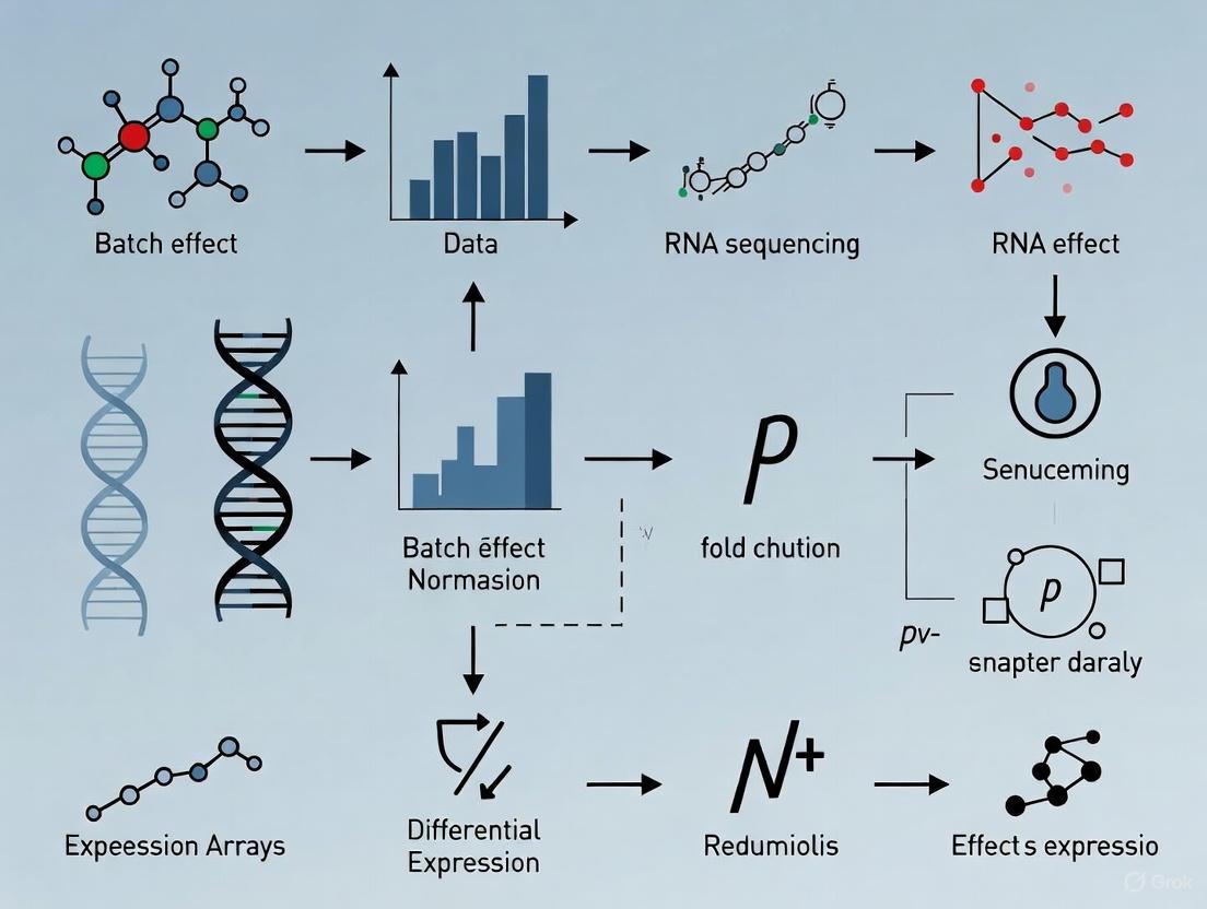
The diagram below illustrates this diagnostic workflow.
Guide 2: Correcting Batch Effects in scRNA-seq Data
For single-cell data, specific methods are required to handle its unique characteristics.
- Objective: To integrate multiple batches of scRNA-seq data, removing technical variation while preserving biological heterogeneity.
- Experimental Protocol:
- Preprocessing: Normalize your raw count data and identify highly variable genes using a standard scRNA-seq pipeline (e.g., in Seurat or Scanpy).
- Method Selection: Choose a batch correction method designed for single-cell data. Based on comprehensive benchmarks, the most effective methods are [3]:
- Harmony: Fast and effective, uses iterative clustering to remove batch effects.
- Seurat Integration: Uses Canonical Correlation Analysis (CCA) and mutual nearest neighbors (MNNs) to find "anchors" between datasets.
- LIGER: Uses integrative non-negative matrix factorization (NMF) to distinguish shared and dataset-specific factors.
- Application: Run the chosen method following its specific tutorial and documentation.
- Validation: Visualize the integrated data using UMAP or t-SNE. After successful correction, cells of the same type from different batches should mix together, while distinct cell types should remain separate.
The following workflow outlines the key steps for single-cell data integration.
Performance Comparison of Batch Effect Correction Algorithms
The table below summarizes the performance of top-performing methods from a large-scale benchmark of scRNA-seq data [3]. Harmony, Seurat 3, and LIGER are generally recommended, with Harmony often favored for its computational speed.
| Method | Key Principle | Best For | Runtime | Data Output |
|---|---|---|---|---|
| Harmony [3] | Iterative clustering in PCA space | General use, large datasets | Fastest | Low-dimensional embedding |
| Seurat 3 [6] [3] | CCA and Mutual Nearest Neighbors (MNN) | Identifying shared cell types across batches | Moderate | Corrected expression matrix |
| LIGER [3] | Integrative Non-negative Matrix Factorization (NMF) | Distinguishing technical from biological variation | Moderate | Factorized matrices |
| ComBat-seq [5] [7] | Empirical Bayes model | Bulk or single-cell RNA-seq count data | Fast | Corrected count matrix |
The Scientist's Toolkit: Key Research Reagent Solutions
The following table details common reagents and materials that are frequent sources of batch effects, emphasizing the need for careful tracking and, where possible, standardization.
| Item | Function | Batch Effect Risk & Mitigation |
|---|---|---|
| Fetal Bovine Serum (FBS) [2] | Provides nutrients and growth factors for cell culture. | High risk. Bioactive components can vary significantly between lots, affecting cell growth and gene expression. Mitigation: Test new lots for performance; use a single lot for an entire study. |
| RNA-Extraction Kits [2] | Isolate and purify RNA from samples. | High risk. Changes in reagent composition or protocol can alter yield and quality. Mitigation: Use the same kit and lot number; if a change is unavoidable, process samples from all groups with both lots to account for the effect. |
| Sequencing Kits & Flow Cells [6] | Prepare libraries and perform sequencing. | High risk. Different lots can have varying efficiencies, leading to batch-specific biases in sequencing depth and quality. Mitigation: Multiplex samples from different biological groups across all sequencing runs. |
| Enzymes (e.g., Reverse Transcriptase) [6] | Converts RNA to cDNA in RNA-seq workflows. | Moderate risk. Variations in enzyme efficiency can affect amplification and library complexity. Mitigation: Use the same reagent batch for a related set of experiments. |
Special Considerations and Limitations
- Unbalanced Designs: Batch effect correction methods can produce misleading results and introduce false positives if your experimental design is unbalanced (e.g., all control samples were processed in one batch and all disease samples in another) [4]. Always aim for a balanced design.
- Over-Correction: Aggressive batch correction can inadvertently remove biologically meaningful signal, especially if there are unknown biological subgroups that are confounded with batch [1] [4]. It is crucial to validate that known biological differences are preserved after correction.
This guide is part of a broader thesis on ensuring data reproducibility in genomic research.
Batch effects are technical variations introduced during experimental processes that are unrelated to the biological signals of interest. They represent a significant challenge in genomics, transcriptomics, proteomics, and metabolomics, potentially leading to misleading outcomes, irreproducible results, and invalidated research findings [8] [2]. This technical support center article details the common sources of batch effects and provides actionable troubleshooting guidance for researchers and drug development professionals.
Batch effects can arise at virtually every stage of a high-throughput study, from initial study design to final data generation [8]. The table below summarizes the most frequently encountered sources of technical variation.
Table 1: Common Sources of Batch Effects in Omics Studies
| Source Category | Specific Examples | Affected Omics Types |
|---|---|---|
| Reagents & Kits | Different lots of RNA-extraction solutions, fetal bovine serum (FBS), enzyme batches for cell dissociation, and reagent quality [8] [9] [2]. | Common to all (Genomics, Transcriptomics, Proteomics, Metabolomics) |
| Instruments & Platforms | Different sequencing machines (e.g., Illumina vs. Ion Torrent), mass spectrometers, laboratory equipment, and changes in hardware calibration [9] [10]. | Common to all |
| Personnel & Protocols | Variations in techniques between different handlers or technicians, differences in sample processing protocols, and deviations in standard operating procedures [10] [5]. | Common to all |
| Lab Conditions | Fluctuations in ambient temperature during cell capture, humidity, ozone levels, and sample storage conditions (e.g., temperature, duration, freeze-thaw cycles) [9] [10]. | Common to all |
| Sample Preparation & Storage | Variables in sample collection, centrifugal forces during plasma separation, time and temperatures prior to centrifugation, and storage duration [8] [2]. | Common to all |
| Sequencing Runs | Processing samples across different days, weeks, or months; different sequencing lanes or flow cells; and variations in PCR amplification efficiency [6] [10]. | Common to all, especially Transcriptomics |
| Flawed Study Design | Non-randomized sample collection, processing batches highly correlated with biological outcomes, and imbalanced cell types across samples [8] [11] [2]. | Common to all |
The following diagram illustrates how these sources introduce variation throughout a typical experimental workflow.
Figure 1: Potential points of batch effect introduction in a high-throughput omics workflow.
How can I detect batch effects in my data?
Before applying corrective measures, it is crucial to assess whether your data suffers from batch effects. Both visual and quantitative methods are available.
Visual Assessment Methods
- Principal Component Analysis (PCA): Perform PCA on your raw data and color the data points by batch. If the top principal components show clear separation of samples by batch rather than by biological condition, this indicates strong batch effects [11] [12] [5].
- t-SNE or UMAP Plots: Visualize your data using t-SNE or UMAP and overlay the batch labels. In the presence of batch effects, cells or samples from different batches will form distinct clusters instead of mixing based on biological similarity (e.g., cell type or disease condition) [11] [12].
- Clustering and Heatmaps: Generate hierarchical clustering dendrograms or heatmaps of your data. If samples cluster primarily by batch instead of by treatment group, it signals a batch effect [11].
Quantitative Metrics
For a less biased assessment, several quantitative metrics can be employed. These are particularly useful for benchmarking the success of batch correction methods.
Table 2: Quantitative Metrics for Assessing Batch Effects
| Metric Name | Description | Interpretation |
|---|---|---|
| kBET (k-nearest neighbor Batch Effect Test) | Tests whether the local neighborhood of a cell matches the global batch composition [9] [13]. | A rejection of the null hypothesis indicates poor local batch mixing. |
| LISI (Local Inverse Simpson's Index) | Measures both batch mixing (Batch LISI) and cell type separation (Cell Type LISI) [9]. | A higher Batch LISI indicates better batch mixing. A higher Cell Type LISI indicates better biological signal preservation. |
| ARI (Adjusted Rand Index) | Measures the similarity between two clusterings (e.g., before and after correction) [12]. | Values closer to 1 indicate better preservation of clustering structure. |
| NMI (Normalized Mutual Information) | Measures the mutual dependence between clustering outcomes and batch labels [12]. | Lower values indicate less dependence on batch, suggesting successful correction. |
| PCR_batch | Percentage of corrected random pairs within batches [12]. | Aids in evaluating the integration of cells from different samples. |
What is the difference between normalization and batch effect correction?
Researchers often confuse these two distinct preprocessing steps. The table below clarifies their different objectives and operational scales.
Table 3: Normalization vs. Batch Effect Correction
| Aspect | Normalization | Batch Effect Correction |
|---|---|---|
| Primary Goal | Adjusts for cell-specific technical biases to make expression counts comparable across cells. | Removes technical variations that are systematically associated with different batches of experiments. |
| Technical Variations Addressed | Sequencing depth (library size), RNA capture efficiency, amplification bias, and gene length [12] [9]. | Different sequencing platforms, processing times, reagent lots, personnel, and laboratory conditions [12]. |
| Typical Input | Raw count matrix (cells x genes) [12]. | Often uses normalized (and sometimes dimensionally-reduced) data, though some methods correct the full expression matrix [12]. |
| Examples | Log normalization, SCTransform, Scran's pooling-based normalization, CLR [9]. | Harmony, Seurat Integration, ComBat, MNN Correct, LIGER [6] [11] [12]. |
The following workflow chart demonstrates how these processes fit into a typical single-cell RNA-seq analysis pipeline.
Figure 2: Placement of normalization and batch effect correction in a standard scRNA-seq analysis workflow.
How do I choose an appropriate batch effect correction method?
Selecting a suitable method depends on your data type, size, and the nature of the biological question. There is no one-size-fits-all solution [8].
Table 4: Commonly Used Batch Effect Correction Methods for Single-Cell RNA-seq
| Method | Underlying Algorithm | Input Data | Strengths | Limitations |
|---|---|---|---|---|
| Harmony [6] [12] [9] | Iterative clustering and linear correction in PCA space. | Normalized count matrix. | Fast, scalable, preserves biological variation well [9] [14]. | Limited native visualization tools [9]. |
| Seurat Integration [6] [12] [9] | Canonical Correlation Analysis (CCA) and Mutual Nearest Neighbors (MNN). | Normalized count matrix. | High biological fidelity, integrates with Seurat's comprehensive toolkit [9]. | Computationally intensive for large datasets [9]. |
| BBKNN [9] | Batch Balanced K-Nearest Neighbors. | k-NN graph. | Computationally efficient, lightweight [9]. | Less effective for complex non-linear batch effects; parameter sensitive [9]. |
| scANVI [9] | Deep generative model (variational autoencoder). | Raw or normalized counts. | Handles complex batch effects; can incorporate cell labels. | Requires GPU; demands technical expertise [9]. |
| ComBat/ComBat-seq [14] [5] | Empirical Bayes framework. | Raw count matrix (ComBat-seq) or normalized data (ComBat). | Established method; good for bulk or single-cell RNA-seq. | Can introduce artifacts; assumptions of linear batch effects [14]. |
| MNN Correct [12] | Mutual Nearest Neighbors. | Normalized count matrix. | Does not require identical cell type compositions. | Computationally demanding; can alter data considerably [12] [14]. |
| LIGER [6] [12] | Integrative non-negative matrix factorization (NMF). | Normalized count matrix. | Effective for large, complex datasets. | Can be aggressive, potentially removing biological signal [14]. |
Practical Correction Protocol
The following step-by-step protocol, adaptable in tools like R or Python, outlines a typical batch correction process using a popular method.
Protocol: Batch Effect Correction using Harmony on scRNA-seq Data
Objective: To integrate multiple single-cell RNA-seq datasets and remove technical batch effects while preserving biological heterogeneity.
Software Requirements: R programming environment, Harmony library, and single-cell analysis toolkit (e.g., Seurat).
Data Preprocessing and Normalization:
- Load your raw count matrices and metadata (containing batch information) into your analysis environment.
- Normalize the data to account for differences in sequencing depth. A common method is log-normalization.
- Select Highly Variable Genes (HVGs) to focus the analysis on genes containing the most biological signal.
- Scale the data and perform principal component analysis (PCA) to obtain a low-dimensional representation.
Assess Batch Effects:
- Visualize the PCA results, coloring cells by their batch of origin. Observe if batches form separate clusters.
- Optionally, compute quantitative metrics like kBET or LISI on the pre-correction PCA embedding to establish a baseline.
Run Harmony Integration:
- Use the
RunHarmonyfunction, providing the PCA embedding and the batch variable (e.g.,batch_var = "processing_date"). - Harmony will iteratively cluster cells and correct the PCA embeddings, returning a new, batch-corrected embedding.
- Use the
Post-Correction Analysis and Validation:
- Use the corrected Harmony embedding to build a k-nearest neighbor (k-NN) graph and perform clustering and UMAP visualization.
- Validate the correction:
- Color the new UMAP by batch. Batches should be well-mixed within biological clusters.
- Color the UMAP by cell type. Distinct cell types should remain separate, confirming biological signals were preserved.
- Be vigilant for signs of over-correction, such as distinct cell types being forced together or a complete overlap of samples from very different biological conditions [11].
What are the signs of over-correction and how can I avoid it?
Over-correction occurs when a batch effect correction method removes not only technical variation but also genuine biological signal. This can be as detrimental as not correcting at all.
Key Signs of Over-Correction:
- Loss of Biological Distinction: Distinct cell types are clustered together on dimensionality reduction plots (UMAP, t-SNE) when they should be separate [11] [12].
- Unrealistic Overlap: A complete overlap of samples originating from very different biological conditions or experiments, especially when minor differences are central to the experimental design [11].
- Compromised Marker Genes: A significant portion of cluster-specific markers are composed of genes with widespread high expression (e.g., ribosomal genes) instead of canonical cell-type-specific markers. There may also be a notable absence of expected differential expression hits [11] [12].
Strategies to Avoid Over-Correction:
- Benchmark Methods: Test multiple batch correction methods on your data. Begin with methods known for good performance, such as Harmony, which has been recommended for being well-calibrated and introducing fewer artifacts [14].
- Use Quantitative Metrics: Employ metrics like LISI that measure both batch mixing (iLISI) and cell type separation (cLISI). A good correction should increase iLISI (better batch mixing) without significantly decreasing cLISI (preserved biological separation) [9].
- Iterative Evaluation: Always compare pre- and post-correction visualizations and metrics. Be critical of results that show perfect mixing at the expense of known biological structure.
Table 5: Essential Experimental and Computational Tools
| Tool / Resource | Function | Relevance to Batch Effect Management |
|---|---|---|
| Standardized Protocols | Detailed, written procedures for sample processing. | Minimizes personnel-induced variation and ensures consistency across experiments and time [6]. |
| Single Reagent Lot | Using the same manufacturing batch of key reagents (e.g., FBS, enzymes) for an entire study. | Prevents a major source of technical variation [8] [6]. |
| Sample Multiplexing | Processing multiple samples together in a single sequencing run using cell hashing or similar techniques. | Reduces confounding of batch and sample identity [11]. |
| Reference Samples | Including control or reference samples in every processing batch. | Provides a technical baseline to monitor and correct for inter-batch variation. |
| Harmony | Computational batch correction tool. | A robust and widely recommended method for integrating single-cell data with minimal artifacts [6] [9] [14]. |
| Seurat | Comprehensive single-cell analysis suite. | Provides a full workflow, including its own high-fidelity integration method [6] [9]. |
| Scanpy | Python-based single-cell analysis toolkit. | Offers multiple integrated batch correction methods like BBKNN and Scanorama [9]. |
| Polly | Data management and processing platform. | Automates batch effect correction and provides "Polly Verified" reports to ensure data quality [12]. |
In the era of large-scale biological data, batch effects represent a fundamental challenge that can compromise the utility of high-throughput genomic, transcriptomic, and proteomic datasets. Batch effects are technical variations introduced into data due to differences in experimental conditions, processing times, personnel, reagent lots, or measurement technologies [15] [2]. These non-biological variations create structured patterns of distortion that permeate all replicates within a processing batch and vary markedly between batches [16]. The consequences range from reduced statistical power to completely misleading findings when batch effects confound true biological signals [2] [16]. This technical support article examines the profound implications of uncorrected batch effects and provides practical guidance for researchers navigating this complex analytical challenge.
FAQ: Understanding Batch Effects
What exactly are batch effects and how do they arise?
Batch effects are technical variations in data that are unrelated to the biological questions under investigation. They arise from differences in experimental conditions across multiple aspects of data generation [2]:
- Sample processing: Variations in personnel, protocols, reagent lots, or equipment across different laboratories or processing days
- Technical platforms: Different sequencing technologies, microarray platforms, or measurement instruments
- Temporal factors: Data collected at different times, even within the same laboratory
- Sample storage: Differences in how samples are collected, prepared, and stored before analysis
The fundamental cause can be partially attributed to fluctuations in the relationship between the actual biological abundance of an analyte and its measured intensity across different experimental conditions [2].
Why are batch effects particularly problematic in genomic studies?
Batch effects have profound negative impacts on genomic studies because they can:
- Reduce statistical power by introducing extra variation that dilutes true biological signals [2] [16]
- Generate false positives when batch effects correlate with outcomes of interest, leading to incorrect conclusions [2]
- Hinder reproducibility across studies and laboratories, potentially resulting in retracted articles and invalidated findings [2]
- Complicate data integration from multiple sources, limiting the value of consortium efforts and meta-analyses [17]
In one documented case, a change in RNA-extraction solution caused a shift in gene-based risk calculations, resulting in incorrect classification for 162 patients, 28 of whom received incorrect or unnecessary chemotherapy regimens [2].
How can I determine if my data has batch effects?
Several approaches can help identify batch effects in your data:
Table 1: Methods for Batch Effect Detection
| Method | Description | Interpretation |
|---|---|---|
| PCA Visualization | Perform PCA on raw data and color points by batch | Separation of samples by batch in top principal components suggests batch effects |
| t-SNE/UMAP Plots | Project data using t-SNE or UMAP and overlay batch labels | Clustering of samples by batch rather than biological factors indicates batch effects |
| Clustering Analysis | Examine dendrograms or heatmaps of samples | Samples clustering by processing batch rather than treatment group signals batch effects |
| Quantitative Metrics | Use metrics like kBET, LISI, or ASW | Statistical measures of batch mixing that reduce human bias in assessment [11] |
What are the signs that I may have over-corrected batch effects?
Over-correction occurs when batch effect removal also eliminates genuine biological signals. Warning signs include [11]:
- Distinct cell types clustering together on dimensionality reduction plots (PCA, t-SNE, UMAP)
- Complete overlap of samples from very different biological conditions or experiments
- Cluster-specific markers comprised mainly of genes with widespread high expression across cell types (e.g., ribosomal genes)
- Loss of expected biological variation that should differentiate sample groups
Troubleshooting Guide: Common Batch Effect Scenarios
Scenario 1: Fully Confounded Study Design
Problem: In a fully confounded design, biological groups completely separate by batches (e.g., all controls in one batch, all cases in another), making it impossible to distinguish biological effects from batch effects [15].
Solutions:
- Remeasurement strategy: If possible, remeasure a subset of samples across batches. Research shows that when between-batch correlation is high, remeasuring even a small subset can rescue most statistical power [18].
- Statistical approaches: Methods like "ReMeasure" specifically address highly confounded case-control studies by leveraging remeasured samples in the maximum likelihood framework [18].
- Prevention: Always design studies with balanced distribution of biological groups across batches when possible.
Scenario 2: Choosing an Inappropriate Correction Method
Problem: Different batch effect correction methods have varying assumptions and performance characteristics. Selecting an inappropriate method can lead to poor correction or over-correction.
Solutions:
- Method benchmarking: Consult comprehensive benchmarking studies that evaluate multiple methods across various data types and scenarios [3] [17].
- Data-type consideration: Choose methods appropriate for your data type and distribution:
- Multiple testing: Try several methods and compare results to ensure robustness.
Scenario 3: Sample Imbalance Across Batches
Problem: Differences in cell type numbers, cell counts per type, and cell type proportions across samples (common in cancer biology) can substantially impact integration results and biological interpretation [11].
Solutions:
- Acknowledge limitations: Recognize that most batch correction methods assume similar cell type compositions across batches.
- Specialized approaches: Consider methods like LIGER, which aims to remove only technical variations while preserving biological differences between batches [3].
- Guidance adherence: Follow refined guidelines for data integration in imbalanced settings, as proposed by Maan et al. (2024) [11].
Experimental Protocols for Batch Effect Management
Protocol 1: Batch Effect Assessment Workflow
- Data Preparation: Begin with raw, unnormalized data from all batches.
- Initial Visualization: Perform PCA and color points by batch identity and biological groups.
- Cluster Analysis: Generate heatmaps and dendrograms to examine sample clustering patterns.
- Quantitative Assessment: Apply metrics like kBET or LISI for objective batch effect quantification.
- Document Findings: Record the extent and nature of batch effects before proceeding with correction.
Figure 1: Batch effect assessment workflow for identifying technical variations in omics data
Protocol 2: Comparative Evaluation of Batch Correction Methods
- Select Multiple Methods: Choose 3-4 methods representing different approaches (e.g., Harmony, Seurat, ComBat).
- Apply Corrections: Implement each method following author recommendations and default parameters.
- Visual Evaluation: Generate UMAP/t-SNE plots of corrected data colored by batch and cell type.
- Quantitative Evaluation: Calculate batch mixing metrics (kBET, LISI) and biological preservation metrics (ASW, ARI).
- Method Selection: Choose the method that best balances batch removal with biological signal preservation.
The Scientist's Toolkit: Batch Effect Correction Methods
Computational Correction Tools
Table 2: Batch Effect Correction Methods and Their Applications
| Method | Approach | Best For | Key Considerations |
|---|---|---|---|
| Harmony | Mixture model-based integration | Single-cell RNA-seq, image-based profiling | Fast runtime, good performance across scenarios [17] [3] |
| ComBat | Empirical Bayes, location-scale adjustment | Microarray, bulk RNA-seq data | Assumes Gaussian distribution after transformation [19] [16] |
| Seurat | CCA or RPCA with mutual nearest neighbors | Single-cell RNA-seq data | Multiple integration options (CCA, RPCA) with different strengths [17] |
| LIGER | Integrative non-negative matrix factorization | Datasets with biological differences between batches | Preserves biological variation while removing technical effects [3] |
| Mutual Nearest Neighbors (MNN) | Nearest neighbor matching across batches | Single-cell RNA-seq | Pioneering approach for single-cell data; basis for several other methods [3] |
| scVI | Variational autoencoder | Large, complex single-cell datasets | Neural network approach; requires substantial computational resources [17] |
Experimental Reagent Solutions
Table 3: Research Reagents and Materials for Batch Effect Mitigation
| Reagent/Material | Function in Batch Effect Control | Implementation Strategy |
|---|---|---|
| Reference Standards | Normalization across batches and platforms | Include identical reference samples in each batch to quantify technical variation |
| Control Samples | Assessment of technical variability | Process positive and negative controls in each batch to monitor performance |
| Standardized Reagent Lots | Reduce batch-to-batch variation | Use the same reagent lots for all samples in a study when possible |
| Sample Multiplexing Kits | Internal batch effect control | Label samples with barcodes and process together to minimize technical variation |
Advanced Topics in Batch Effect Correction
Batch Effects in Emerging Technologies
As new technologies evolve, they present unique batch effect challenges:
Single-cell RNA sequencing: scRNA-seq data suffers from higher technical variations than bulk RNA-seq, including lower RNA input, higher dropout rates, and greater cell-to-cell variation, making batch effects more severe [2].
Image-based profiling: Technologies like Cell Painting, which extracts morphological features from cellular images, face batch effects from different microscopes, staining concentrations, and cell growth conditions across laboratories [17] [20].
Multi-omics integration: Combining data from different omics layers (genomics, transcriptomics, proteomics) introduces additional complexity as each data type has different distributions, scales, and batch effect characteristics [2].
The Role of Experimental Design in Batch Effect Prevention
Proper experimental design remains the most effective strategy for managing batch effects:
- Balance and randomization: Distribute biological groups of interest equally across all processing batches [15] [16]
- Batch recording: Meticulously document all potential batch variables (processing date, personnel, reagent lots, instrument ID)
- Reference samples: Include technical replicates and reference materials in each batch to facilitate downstream correction
- Block designs: Structure experiments so that biological comparisons of interest are made within rather than between batches
Figure 2: Experimental design strategies to prevent batch effects and ensure valid biological conclusions
Batch effects represent a fundamental challenge in modern biological research that cannot be ignored or easily eliminated. The consequences of uncorrected batches range from reduced statistical power to completely misleading biological conclusions, with potentially serious implications for both basic research and clinical applications. Successful navigation of this landscape requires a multi-faceted approach: vigilant experimental design to minimize batch effects at source, comprehensive assessment to quantify their impact, appropriate correction methods tailored to specific data types and research questions, and careful evaluation to avoid over-correction that removes biological signal along with technical noise. As technologies evolve and datasets grow in size and complexity, continued development and benchmarking of batch effect correction methods will remain essential for ensuring the reliability and reproducibility of biological findings.
A technical support guide for genomic researchers
What are batch effects and why is detecting them crucial?
In transcriptomics, a batch effect refers to systematic, non-biological variation introduced into gene expression data by technical inconsistencies. These can arise from differences in sample collection, library preparation, sequencing machines, reagent lots, or personnel [21].
If undetected, these technical variations can obscure true biological signals, leading to misleading conclusions, false positives in differential expression analysis, or missed discoveries [21]. Visual diagnostic tools like PCA, t-SNE, and UMAP provide a first and intuitive way to detect these unwanted patterns.
How do I use PCA, t-SNE, and UMAP to spot batch effects?
The core principle is simple: in the presence of a strong batch effect, cells or samples will cluster by their technical batch rather than by their biological identity (e.g., cell type or treatment condition) [11].
The table below summarizes the standard approach for each method.
| Method | How to Perform Detection | What Indicates a Batch Effect? |
|---|---|---|
| PCA | Perform PCA on raw data and create scatter plots of the top principal components (e.g., PC1 vs. PC2) [11]. | Data points separate into distinct groups based on batch identity along one or more principal components [11]. |
| t-SNE / UMAP | Generate t-SNE or UMAP plots and color the data points by their batch of origin [11]. | Clear separation of batches into distinct, non-overlapping clusters on the 2D plot [21] [11]. |
The following workflow diagram outlines the key steps for visual diagnosis and subsequent correction of batch effects.
My data shows batch effects. What correction method should I use?
Several statistical and machine learning methods have been developed to correct for batch effects. The choice of method can depend on your data type (e.g., bulk vs. single-cell RNA-seq) and the complexity of the batch effect.
Recent independent benchmarking studies have compared the performance of various methods. The following table summarizes findings from a 2025 study that compared eight widely used methods for single-cell RNA-seq data [22].
| Method | Reported Performance | Key Notes |
|---|---|---|
| Harmony | Consistently performed well in all tests; only method recommended by the study [22]. | Often noted for fast runtime in other benchmarks [11]. |
| ComBat | Introduced measurable artifacts in the test setup [22]. | Uses an empirical Bayes framework; widely used but requires known batch info [21]. |
| ComBat-Seq | Introduced measurable artifacts in the test setup [22]. | Variant for RNA-Seq raw count data [23]. |
| Seurat | Introduced measurable artifacts in the test setup [22]. | Often used in single-cell analyses; earlier versions used CCA, later versions use MNNs [24]. |
| BBKNN | Introduced measurable artifacts in the test setup [22]. | A fast method that works by creating a batch-balanced k-nearest neighbour graph [25]. |
| MNN | Performed poorly, often altering data considerably [22]. | Mutual Nearest Neighbors; a foundational algorithm used by other tools [24]. |
| SCVI | Performed poorly, often altering data considerably [22]. | A neural network-based approach (Variational Autoencoder) [24]. |
| LIGER | Performed poorly, often altering data considerably [22]. | Based on integrative non-negative matrix factorization [11]. |
Note: Another large-scale benchmark (Luecken et al., 2022) suggested that scANVI (a neural network-based method) performs best, while Harmony is a good but less scalable option [11]. It is advisable to test a few methods on your specific dataset.
How can I be sure I haven't over-corrected and removed biology?
Over-correction is a valid concern, where the correction method removes true biological variation along with the technical noise [21]. Watch for these indicative signs:
- Distinct Cell Types Merge: After correction, previously separate cell types are clustered together on your UMAP/t-SNE plot [11].
- Implausible Overlap: A complete overlap of samples from very different biological conditions (e.g., healthy and diseased) where some differences are expected [11].
- Non-informative Markers: Cluster-specific markers identified after correction are dominated by genes with widespread high expression (e.g., ribosomal genes) instead of biologically meaningful markers [11].
If you suspect over-correction, try a less aggressive correction method or adjust its parameters.
A Researcher's Toolkit: Key Metrics for Quantifying Batch Effects
While visual tools are essential for a first pass, quantitative metrics provide an objective assessment of batch effect strength and correction quality. The table below lists key metrics used in the field [26] [21] [24].
| Metric Name | Type | What It Measures | Interpretation |
|---|---|---|---|
| Average Silhouette Width (ASW) | Cell type-specific | How well clusters are separated and cohesive. Higher values indicate better-defined clusters [26] [21]. | Values close to 1 indicate tight, well-separated clusters. Batch effects reduce ASW [21]. |
| k-Nearest Neighbour Batch Effect Test (kBET) | Cell type-specific / Cell-specific | Tests if batch proportions in a cell's neighbourhood match the global proportions [26] [21]. | A high acceptance rate indicates good batch mixing within cell types [21] [24]. |
| Local Inverse Simpson's Index (LISI) | Cell-specific | The effective number of batches in a cell's neighbourhood [26] [21]. | Higher LISI scores indicate better mixing, with an ideal score equal to the number of batches [21]. |
| Cell-specific Mixing Score (cms) | Cell-specific | Tests if distance distributions in a cell's neighbourhood are batch-specific [26]. | A p-value indicating the probability of observed differences assuming no batch effect. Lower p-values suggest local batch bias [26]. |
| Graph Connectivity (GC) | Cell type-specific | The fraction of cells that remain connected in a graph after batch correction [24]. | Higher values (closer to 1) indicate better preservation of biological group structure [24]. |
Essential Materials and Reagents for scRNA-seq Batch Effect Investigation
The following table details key reagents and computational tools frequently mentioned in batch effect research.
| Item / Tool Name | Function / Description |
|---|---|
| Harmony | A robust batch correction algorithm that uses PCA and iterative clustering to integrate data across batches [22] [24]. |
| Seurat | A comprehensive R toolkit for single-cell genomics, which includes data integration functions [22] [24]. |
| CellMixS | An R/Bioconductor package that provides the cell-specific mixing score (cms) to quantify and visualize batch effects [26]. |
| BBKNN | A batch effect removal tool that quickly computes a batch-balanced k-nearest neighbour graph [25]. |
| scGen / FedscGen | A neural network-based method (VAE) for batch correction. FedscGen is a privacy-preserving, federated version [24]. |
| pyComBat | A Python implementation of the empirical Bayes methods ComBat and ComBat-Seq for correcting batch effects [23]. |
Experimental Protocol: A Standard Workflow for Visual Batch Effect Diagnosis
This protocol provides a step-by-step guide for detecting batch effects using visual tools, as commonly implemented in tools like Scanpy or Seurat.
Objective: To visually assess the presence of technical batch effects in a single-cell RNA sequencing dataset.
Materials:
- A compiled single-cell dataset (e.g., an AnnData object in Scanpy or a Seurat object) containing cells from multiple batches.
- Bioinformatics environment with Python (Scanpy, NumPy) or R (Seurat) installed.
Procedure:
- Data Preprocessing: Perform standard preprocessing on your raw count matrix. This typically includes quality control filtering, normalization, and log-transformation. Identify highly variable genes.
- Dimensionality Reduction (PCA):
- Scale the data to unit variance and zero mean.
- Perform Principal Component Analysis (PCA) on the scaled data of highly variable genes.
- Visualization: Create a scatter plot of the first two principal components (PC1 vs. PC2). Color the data points by their batch identifier (e.g., sequencing run, donor).
- Interpretation: Observe if points cluster strongly by batch. Proceed to the next step regardless.
- Non-Linear Embedding (UMAP/t-SNE):
- Construct a k-nearest neighbour (k-NN) graph based on the top principal components (e.g., first 20-50 PCs).
- Generate a UMAP (or t-SNE) plot from this k-NN graph.
- Visualization: Create the UMAP plot and color the data points by batch. Generate a second UMAP plot colored by cell type or biological condition.
- Interpretation: Compare the two plots. In the "batch" plot, check for strong, separate clusters based on batch. In the "cell type" plot, check if the same cell type from different batches forms separate clusters instead of mixing together.
- Documentation and Decision:
- Save all plots.
- If visual inspection reveals strong batch clustering, proceed to batch correction using a method of choice (see FAQ above). After correction, always repeat steps 2 and 3 to validate that the batch effect has been reduced and biological structures are preserved.
This workflow is encapsulated in the following diagram, which also includes the iterative validation step after correction.
What are the primary formal statistical tests for batch effect detection?
Several formal statistical tests exist to diagnose batch effects, moving beyond visual inspection of PCA plots. The table below summarizes the key methods:
| Method Name | Underlying Principle | Key Metric | Interpretation |
|---|---|---|---|
| findBATCH [27] | Probabilistic Principal Component and Covariates Analysis (PPCCA) | 95% Confidence Intervals (CIs) for batch effect on each probabilistic PC | pPCs with 95% CIs not including zero have a significant batch effect |
| Guided PCA (gPCA) [28] | Guided Singular Value Decomposition (SVD) using a batch indicator matrix | δ statistic (proportion of variance due to batch) | δ near 1 implies a large batch effect; significance is assessed via permutation testing (p-value) |
| Principal Variance Component Analysis (PVCA) [27] [29] | Hybrid approach combining PCA and variance components analysis | Proportion of variance explained by the batch factor | A higher proportion indicates a greater influence of batch effects on the data |
Can you provide a protocol for implementing the findBATCH and gPCA tests?
Experimental Protocol: Statistical Testing for Batch Effects
A. Implementation of findBATCH using the exploBATCH R Package
- Data Pre-processing and Normalization: Independently pre-process and normalize each individual dataset according to the technology used (e.g., microarray, RNA-seq). [27]
- Data Pooling: Pool the processed datasets based on common identifiers, such as gene names or probes. [27]
- Optimal Component Selection: Run the
findBATCHfunction. It will first select the optimal number of probabilistic Principal Components (pPCs) based on the highest Bayesian Information Criterion (BIC) value. These pPCs explain the majority of the data variability. [27] - Statistical Testing and Visualization: The function computes the estimated batch effect (as a regression coefficient) and its 95% Confidence Interval for each pPC. Results are typically displayed in a forest plot. [27]
- Interpretation: Identify pPCs where the 95% CI for the batch effect does not include zero. These are the components significantly associated with batch effects. [27]
B. Implementation of Guided PCA (gPCA) using the gPCA R Package
- Batch Indicator Matrix: Create a batch indicator matrix (
Y) where rows represent samples and columns represent different batches. [28] - Perform gPCA: Conduct a guided PCA on the matrix
X'Y, whereXis your centered genomic data matrix (e.g., gene expression). This guides the analysis to find directions of variation associated with the predefined batches. [28] - Calculate the δ Statistic: Compute the test statistic
δ, which is the ratio of the variance explained by the first principal component from gPCA to the variance explained by the first principal component from traditional, unguided PCA. [28]δ = (Variance of PC1 from gPCA) / (Variance of PC1 from unguided PCA) - Permutation Test for Significance:
- Permute the batch labels of the samples (e.g., 1000 times).
- For each permutation, recalculate the δ statistic (
δ_p). - The p-value is the proportion of permuted
δ_pvalues that are greater than or equal to the observed δ value from the original data. [28]
- Interpretation: A significant p-value (e.g., < 0.05) indicates the presence of a statistically significant batch effect in the data. [28]
What are the common metrics for evaluating batch effect correction performance?
After applying a batch correction method, its performance can be quantitatively evaluated using the following sample-based and feature-based metrics:
| Metric Category | Metric Name | Description | Application Context |
|---|---|---|---|
| Sample-Based Metrics | Signal-to-Noise Ratio (SNR) [29] | Evaluates the resolution in differentiating known biological groups (e.g., using PCA). Higher SNR indicates better preservation of biological signal. | Used when sample group labels are known. |
| Principal Variance Component Analysis (PVCA) [29] | Quantifies the proportion of total variance in the data explained by biological factors versus batch factors. A successful correction reduces the variance component for batch. | General purpose for partitioned variance. | |
| Feature-Based Metrics | Coefficient of Variation (CV) [29] | Measures the variability of a feature (e.g., a gene) across technical replicates within and between batches. Lower CV after correction indicates improved precision. | Requires technical replicates. |
| Matthews Correlation Coefficient (MCC) & Pearson Correlation (RC) [29] | Assess the accuracy of identifying Differentially Expressed Genes/Proteins (DEGs/DEPs). MCC is more robust for unbalanced designs. Used with simulated data where the "truth" is known. | Benchmarking with simulated data. |
What statistical pitfalls should I be aware of during batch correction?
A major consideration is the choice between a one-step and a two-step correction process, which can significantly impact downstream statistical inference. [30]
- One-Step Correction: Batch variables are included directly in the statistical model during the primary analysis (e.g., differential expression). This is statistically sound but can be inflexible for complex downstream analyses. [30]
- Two-Step Correction: Batch effects are removed in a preprocessing step, and the "cleaned" data is used for all downstream analyses. While popular and flexible, this approach has a critical pitfall: the correction process introduces a correlation structure between samples within the same batch. [30]
- The Problem: If this induced correlation is ignored in downstream analyses (e.g., by using a standard linear model that assumes independent samples), it can lead to either exaggerated significance (increased false positives) or diminished significance (loss of power). This is especially problematic in unbalanced designs where biological groups are not uniformly distributed across batches. [30]
- The Solution: If using a two-step method like ComBat, one proposed solution is to use the ComBat+Cor approach. This involves estimating the sample correlation matrix of the batch-corrected data and incorporating it into the downstream model using Generalized Least Squares (GLS) to account for the dependencies. [30]
| Item / Resource | Function / Application |
|---|---|
| R Statistical Software | The primary environment for implementing most statistical batch effect tests and corrections. [27] [28] |
exploBATCH R Package |
Provides the implementation for the findBATCH (detection) and correctBATCH (correction) methods based on PPCCA. [27] |
gPCA R Package |
Provides functionality to perform guided PCA and the associated statistical test for batch effects. [28] |
sva / ComBat-seq R Package |
Contains the ComBat and ComBat-seq algorithms for two-step batch effect correction, widely used as a standard. [31] [7] |
| Reference Materials (e.g., Quartet Project) | Well-characterized control samples (like the Quartet protein reference materials) profiled across multiple batches and labs to benchmark and evaluate batch effect correction methods. [29] |
| Simulated Data with Known Truth | Datasets with built-in batch effects and known differential expression patterns, used for controlled method validation and calculation of metrics like MCC. [29] |
A Methodologist's Toolkit: Choosing and Applying the Right Correction Algorithm
The integration of large-scale genomics data has become fundamental to modern biological research and drug development. However, this integration is routinely hindered by unwanted technical variations known as batch effects—systematic differences between datasets generated under different experimental conditions, times, or platforms [32]. These effects can obscure true biological signals, reduce statistical power, and potentially lead to false positive findings if not properly addressed [33] [34].
The Empirical Bayes framework ComBat has emerged as a powerful approach for correcting these technical artifacts. Originally developed for microarray gene expression data, ComBat estimates and removes additive and multiplicative batch effects using an empirical Bayes approach that effectively borrows information across features [35]. This method has seen widespread adoption across genomic technologies due to its ability to handle small sample sizes while avoiding over-correction.
More recently, the field has witnessed the development of ComBat-met, a specialized extension designed to address the unique characteristics of DNA methylation data [32]. Unlike other genomic data types, DNA methylation is quantified as β-values (methylation percentages) constrained between 0 and 1, often exhibiting skewness and over-dispersion that violate the normality assumptions of standard ComBat [32] [34]. ComBat-met employs a beta regression framework specifically tailored to these distributional properties, representing a significant evolution in the ComBat methodology for epigenomic applications.
ComBat-met: Technical Framework and Implementation
Core Methodology
ComBat-met addresses the fundamental limitation of standard ComBat when applied to DNA methylation data. Traditional ComBat assumes normally distributed data, making it suboptimal for β-values that are proportion measurements bounded between 0 and 1 [32]. The ComBat-met framework introduces several key innovations:
Beta Regression Model: Instead of using normal distribution assumptions, ComBat-met models β-values using a beta distribution parameterized by mean (μ) and precision (φ) parameters [32]. This better captures the characteristic distribution of methylation data.
Quantile-Matching Adjustment: The adjustment procedure calculates batch-free distributions and maps the quantiles of the estimated distributions to their batch-free counterparts [32]. This non-parametric approach preserves the distributional properties of the corrected data.
Reference-Based Option: Unlike the standard ComBat which typically aligns batches to an overall mean, ComBat-met provides the option to adjust all batches to a designated reference batch, preserving the technical characteristics of a specific dataset [32].
The method can be represented by the following statistical model:
Let ( y_{ij} ) denote the β-value of a feature in sample ( j ) from batch ( i ). The beta regression model is defined as:
[ \begin{align} y_{ij} &\sim \text{Beta}(\mu_{ij}, \phi_i) \ \text{logit}(\mu_{ij}) &= \alpha + X\beta + \gamma_i \end{align} ]
Where ( \alpha ) represents the common cross-batch average, ( X\beta ) captures biological covariates, and ( \gamma_i ) represents the batch-associated additive effect [32].
Implementation Workflow
The following diagram illustrates the complete ComBat-met workflow from data input through batch-corrected output:
Figure 1: ComBat-met analysis workflow showing the sequence from raw data input through processing steps to corrected output.
Practical Implementation
For researchers implementing ComBat-met, the following code example demonstrates the basic function call using the R package:
The package supports advanced features including reference-batch correction and parallelization to improve computational efficiency with large datasets [36].
Performance Benchmarking and Comparative Analysis
Experimental Design for Method Validation
To validate the performance of ComBat-met, comprehensive benchmarking analyses were conducted using simulated data with known ground truth. The simulation setup included:
- Dataset Characteristics: 1000 features with a balanced design involving two biological conditions and two batches across 20 samples [32].
- Differential Methylation: 100 out of 1000 features were simulated as truly differentially methylated, with methylation percentages higher under condition 2 than condition 1 by 10% [32].
- Batch Effects: Introduction of varying batch effect magnitudes, with methylation percentages in one batch differing by 0%, 2%, 5%, or 10%, and precision parameters varying from 1- to 10-fold between batches [32].
The simulation was repeated 1000 times, followed by differential methylation analysis. Performance was assessed using true positive rates (TPR) and false positive rates (FPR), calculated as the proportion of significant features among those that were and were not truly differentially methylated, respectively [32].
Comparative Performance Results
The table below summarizes the quantitative performance comparison between ComBat-met and alternative batch correction methods based on simulation studies:
Table 1: Performance comparison of batch correction methods for DNA methylation data
| Method | Core Approach | Median TPR | Median FPR | Key Strengths | Key Limitations |
|---|---|---|---|---|---|
| ComBat-met | Beta regression with quantile matching | Highest | Controlled (0.05) | Preserves β-value distribution; Optimized for methylation data | Requires sufficient sample size per batch |
| M-value ComBat | Logit transformation followed by standard ComBat | Moderate | Controlled | Widely available; Familiar framework | Distributional inaccuracy for extreme β-values |
| SVA | Surrogate variable analysis on M-values | Moderate | Variable | Handles unknown batch effects | Can remove biological signal if confounded |
| Include Batch in Model | Direct covariate adjustment in linear model | Lower | Controlled | Simple implementation | Limited for complex batch structures |
| BEclear | Latent factor models | Lower | Slightly elevated | Directly models β-values | Less effective for strong batch effects |
| RUVm | Control-based removal of unwanted variation | Moderate | Variable | Uses control features | Requires appropriate control probes |
Note: TPR = True Positive Rate; FPR = False Positive Rate. Performance metrics based on simulated data with known ground truth [32] [36].
Application to TCGA Data
The practical utility of ComBat-met was demonstrated through application to breast cancer methylation data from The Cancer Genome Atlas (TCGA). Results showed that:
- Variance Explanation: ComBat-met consistently achieved the smallest percentage of batch-associated variation in both normal and tumor samples compared to alternative methods [36].
- Classification Improvement: In machine learning applications, batch adjustment using ComBat-met consistently improved classification accuracy of normal versus cancerous samples when using randomly selected methylation probes [36].
- Biological Signal Recovery: The method effectively recovered biologically meaningful signals while removing technical variations, as validated through known breast cancer subtype classifications [32].
Troubleshooting Guide: Common Implementation Challenges
False Positive Results and p-value Inflation
Issue: Unexpectedly high numbers of significant results after batch correction, potentially indicating false positives.
Background: Several studies have reported that standard ComBat can systematically introduce false positive findings in DNA methylation data under certain conditions [33]. One study demonstrated that applying ComBat to randomly generated data produced alarming numbers of false discoveries, even with Bonferroni correction [33].
Solutions:
- Validate with Simulated Null Data: Generate data with no biological signal but similar experimental structure to assess baseline false positive rates [33].
- Check Batch-Condition Confounding: Ensure biological conditions are not completely confounded with batch structure, as this makes separation of technical and biological variance difficult [34].
- Avoid Over-Correction: Limit the number of batch factors corrected, as increasing the number of corrected factors exponentially increases false positive rates [33].
- Use Appropriate Sample Sizes: Larger sample sizes reduce but do not completely prevent false positive inflation [33].
Data Distribution Violations
Issue: Poor performance when data distribution assumptions are violated.
Background: Standard ComBat assumes normality, making it inappropriate for raw β-values. Even with M-value transformation, distributional issues may persist [32] [34].
Solutions:
- Use Distribution-Appropriate Methods: Apply ComBat-met instead of standard ComBat for β-values to respect their bounded nature [32].
- Diagnose Distribution Fit: Check Q-Q plots and distribution diagnostics before and after correction.
- Consider Alternative Transformations: For standard ComBat, ensure proper transformation to M-values, though ComBat-met eliminates this requirement [32].
Reference Batch Selection
Issue: Suboptimal performance when using reference batch adjustment.
Background: ComBat-met allows alignment to a reference batch, but inappropriate reference selection can introduce biases [32].
Solutions:
- Choose Technically Superior Batches: Select reference batches with highest data quality based on quality control metrics.
- Consider Biological Representation: Ensure reference batch adequately represents biological groups of interest.
- Validate Choice Sensitivity: Test multiple reference batches to assess result robustness.
Probe-Specific Batch Effects
Issue: Residual batch effects in specific probes after correction.
Background: Certain methylation probes are particularly susceptible to batch effects due to sequence characteristics, with 4649 probes consistently requiring high amounts of correction across datasets [34].
Solutions:
- Filter Problematic Probes: Consider removing persistently problematic probes identified in previous studies [34].
- Apply Probe-Specific Adjustments: Use methods that account for probe-specific technical characteristics.
- Implement Post-Correction Diagnostics: Check for residual batch effects stratified by probe type.
Essential Research Reagents and Computational Tools
Table 2: Key software tools and resources for ComBat and ComBat-met implementation
| Tool/Resource | Function | Application Context | Implementation |
|---|---|---|---|
| ComBat-met | Beta regression-based batch correction | DNA methylation β-values | R package: ComBat_met() function |
| sva Package | Standard ComBat implementation | Gene expression, M-values | R package: combat() function |
| ChAMP Pipeline | Integrated methylation analysis | EPIC/450K array data | Includes ComBat as option |
| methylKit | DNA methylation analysis | Simulation and differential analysis | Used for performance benchmarking |
| betareg | Beta regression modeling | General proportional data | Core dependency for ComBat-met |
| TCGA Data | Real-world validation dataset | Breast cancer and other malignancies | Publicly available from NCI |
Advanced Experimental Protocols
Comprehensive Batch Effect Correction Protocol
For researchers implementing batch effect correction in DNA methylation studies, the following detailed protocol ensures robust results:
Pre-correction Quality Control
- Perform principal component analysis (PCA) to visualize batch-associated clustering
- Calculate variance explained by batch versus biological factors
- Identify potential batch-condition confounding
- Check for missing data patterns correlated with batch
Method Selection Criteria
- Use ComBat-met for β-values without transformation
- Consider M-value ComBat only for small datasets when ComBat-met is computationally prohibitive
- Apply reference batch correction when aligning to a specific dataset
- Use cross-batch averaging for balanced multi-batch studies
Parameter Optimization
- For small sample sizes (n < 10 per batch), enable parameter shrinkage
- For large datasets, implement parallel processing to reduce computation time
- Adjust model specifications to include biological covariates when appropriate
Post-correction Validation
- Re-run PCA to confirm batch effect removal
- Verify biological signals are preserved using known positive controls
- Check that corrected values maintain appropriate distribution (β-values between 0-1)
- Test sensitivity to parameter variations
Neural Network Validation Protocol
To evaluate the impact of batch correction on downstream predictive models, the following protocol can be implemented:
Probe Selection: Randomly select three methylation probes in each iteration to simulate minimal, unbiased feature sets [36].
Classifier Architecture: Implement a feed-forward, fully connected neural network with two hidden layers for classifying normal versus cancerous samples [36].
Performance Assessment: Calculate and compare accuracy for models trained on unadjusted versus batch-adjusted data across multiple iterations [36].
This approach demonstrates the practical utility of batch correction in improving predictive modeling performance while avoiding cherry-picking of features that might artificially inflate performance metrics.
Critical Methodological Considerations
When to Avoid ComBat Methods
Despite their utility, ComBat methods should be avoided in certain scenarios:
- Complete Confounding: When batch and biological conditions are perfectly confounded, no statistical method can reliably separate technical from biological variance [34].
- Extreme Small Sample Sizes: With fewer than 5 samples per batch, parameter estimates become unstable, potentially introducing more artifacts than they remove [33].
- Inappropriate Data Types: Standard ComBat should not be applied to β-values without transformation, as distributional assumptions are violated [32].
Emerging Alternatives and Extensions
The field continues to evolve with new approaches addressing ComBat limitations:
- iComBat: An incremental framework for batch effect correction in DNA methylation array data, particularly useful for repeated measurements [37].
- Harmonization Methods: Approaches like those used in medical imaging may offer alternative strategies for certain data types [35].
- Cross-Platform Validation: Always validate findings using multiple batch correction approaches to ensure result robustness.
Visual Decision Framework
The following diagram provides a systematic approach for selecting appropriate batch correction strategies based on data characteristics:
Figure 2: Decision framework for selecting appropriate batch correction methods based on data characteristics and experimental design.
Frequently Asked Questions (FAQs)
1. When should I NOT apply batch correction to my single-cell RNA-seq data? Batch correction is not always appropriate. You should avoid or carefully evaluate using it when:
- Your "batches" are actually different biological conditions, treatments, or time points that you want to compare. Over-correction can remove the biological variation you are trying to study [38].
- You are analyzing a homogeneous population of cells (e.g., a single cell line) with limited inherent biological variation to anchor the integration, as this can lead to spurious alignment [38].
- Your goal is to identify dataset-specific cell states or population structures, as aggressive integration can mask these differences [39].
2. My data is over-corrected after using Seurat's CCA. What can I do? Seurat's CCA method can sometimes be overly aggressive in removing variation. A recommended alternative is to use Seurat's RPCA (Reciprocal PCA) workflow, which is designed to prioritize the conservation of biological variation over complete batch removal [38]. Benchmarking studies have shown that different methods balance batch removal and bio-conservation differently, so trying a less aggressive method like RPCA, Scanorama, or scVI may be beneficial [40].
3. How do I choose between Harmony, Seurat, and LIGER for my project? The choice depends on your data and goals. The table below summarizes key characteristics based on independent benchmarking [40]:
| Method | Key Strength | Optimal Use Case |
|---|---|---|
| Harmony | Fast, sensitive, accurate; performs well on scATAC-seq data [41] [40] | Large datasets; integrating data from multiple donors, tissues, or technologies [41]. |
| Seurat (CCA & RPCA) | Well-established, comprehensive workflow; RPCA prioritizes bio-conservation [38] [40] | Standard integration tasks; when a full-featured pipeline is desired [40]. |
| LIGER | Identifies shared and dataset-specific factors; good for cross-species and multi-omic integration [39] [42] [40] | Comparing and contrasting datasets; multi-modal integration (e.g., RNA-seq + ATAC-seq) [39] [42]. |
4. Should I use SCTransform normalization before integration?
While SCTransform is a powerful normalization method, its use before integration requires caution. The SCTransform method can be used, but it is not a direct substitute for batch correction algorithms like Harmony or IntegrateData [43]. For some integration methods, using standard log-normalization may be more straightforward and equally effective [38]. It is critical to follow the specific requirements of your chosen integration method, as some may not accept SCTransform-scaled data [40].
Troubleshooting Guides
Issue 1: Poor Mixing After Integration
Problem: After running an integration method (e.g., Harmony, Seurat), cells from different batches still form separate clusters in visualizations like UMAP.
Solutions:
- Check Biological Overlap: Confirm that the same cell types are present across all batches. Integration methods can only align shared cell types or states [38].
- Adjust Method Parameters: Increase the strength of the integration. In Harmony, you can increase the
thetaparameter, which controls the diversity penalty, to encourage better mixing. Re-run the algorithm with more iterations if it did not converge [44]. - Try an Alternative Method: If one method fails, try another. Benchmarking has shown that no single method outperforms all others in every scenario [40]. For example, if Seurat's CCA is too aggressive, try RPCA or Scanorama [38] [40].
Issue 2: Loss of Biological Variation After Integration
Problem: Biologically distinct cell populations (e.g., different treatment conditions or known subtypes) are artificially merged after integration.
Solutions:
- Re-evaluate the Need for Correction: This is a classic sign of over-correction. If the "batch" you are correcting for is a key biological variable, you should not integrate across it [38].
- Use a Less Aggressive Workflow: Switch to an integration method known to better preserve biological variation. Seurat's RPCA and Scanorama have been benchmarked to prioritize bio-conservation [38] [40].
- Validate with Marker Genes: Always check the expression of known marker genes for the lost populations in the integrated space to confirm they have been erroneously merged [45].
Issue 3: Harmony Fails to Converge or is Slow
Problem: Harmony throws warnings like "did not converge in 25 iterations" or runs very slowly on large datasets.
Solutions:
- Increase Iterations: Set the
max.iter.harmonyparameter to a higher value (e.g., 50 or 100) to allow the algorithm more time to converge [44]. - Optimize Performance:
- Ensure your R installation is linked with OPENBLAS instead of BLAS, as this can substantially speed up Harmony's performance [46].
- By default, Harmony turns off multi-threading to avoid inefficient CPU usage. For very large datasets (>1 million cells), you can try gradually increasing the
ncoresparameter to utilize multiple threads [46].
Experimental Protocols & Workflows
Generic Workflow for Single-Cell Data Integration
The following diagram outlines the standard steps for integrating single-cell datasets, which is common to most analysis pipelines.
Detailed Method-Specific Protocols
1. Harmony Integration within a Seurat Workflow This protocol details how to run Harmony on a Seurat object after standard preprocessing.
- Input: A Seurat object containing multiple datasets, with PCA computed.
- Code Example:
- Key Parameters:
2. LIGER for Multi-Modal Integration LIGER uses integrative Non-Negative Matrix Factorization (iNMF) to jointly define shared and dataset-specific factors.
- Input: Multiple normalized count matrices (e.g., from scRNA-seq and snATAC-seq).
- Workflow Diagram:
- Key Parameters:
k: The number of factors (metagenes). This is a critical parameter that determines the granularity of the inferred biological signals [39].lambda: The tuning parameter that adjusts the relative strength of dataset-specific versus shared factors. A higherlambdavalue yields more dataset-specific factors [42].
The Scientist's Toolkit: Essential Research Reagents & Materials
The following table lists key computational "reagents" and tools essential for performing single-cell data integration.
| Item | Function & Explanation | Relevant Context |
|---|---|---|
| Cell Ranger | A set of analysis pipelines from 10x Genomics that process raw sequencing data (FASTQ) into aligned reads and a feature-barcode matrix. This is the foundational starting point for many analyses [47]. | Data Preprocessing |
| Highly Variable Genes (HVGs) | A filtered set of genes that exhibit high cell-to-cell variation. Focusing on HVGs reduces noise and computational load, and has been shown to improve the performance of data integration methods [40]. | Normalization & Feature Selection |
| PCA (Principal Component Analysis) | A linear dimensionality reduction technique. It is the default method in many workflows to create an initial low-dimensional embedding of the data, which is often used as direct input for integration algorithms like Harmony [41] [44]. | Dimensionality Reduction |
| UMAP (Uniform Manifold Approximation and Projection) | A non-linear dimensionality reduction technique used widely for visualizing single-cell data in 2D or 3D. It allows researchers to visually assess the effectiveness of integration and the structure of cell clusters [47]. | Visualization & Exploration |
| Benchmarking Metrics (e.g., kBET, ASW, LISI) | A set of quantitative metrics used to evaluate integration quality. They separately measure batch effect removal (e.g., kBet, iLISI) and biological conservation (e.g., cell-type ASW, cLISI), providing an objective score for method performance [40]. | Result Validation |
Batch effects represent systematic technical variations between datasets generated under different conditions (e.g., different sequencing runs, protocols, or laboratories). These non-biological variations can obscure true biological signals and lead to incorrect conclusions in single-cell RNA sequencing (scRNA-seq) analysis [9]. Traditional batch effect correction methods often fail to preserve the intrinsic order of gene expression levels within cells, potentially disrupting biologically meaningful patterns crucial for downstream analysis [48].
Order-preserving batch effect correction addresses this limitation by maintaining the relative rankings of gene expression levels during the correction process. This approach ensures that biologically significant expression patterns remain intact after integration, providing more reliable data for identifying cell types, differential expression, and gene regulatory relationships [48].
Key Concepts and Terminology
Batch Effect: Systematic technical differences between datasets that are not due to biological variation. These can stem from differences in sample preparation, sequencing runs, reagents, or instrumentation [9].
Order-Preserving Feature: A property of batch effect correction methods that maintains the relative rankings or relationships of gene expression levels within each batch after correction [48].
Monotonic Deep Learning Network: A specialized neural network architecture that preserves the order relationships in data during transformation, making it particularly suitable for order-preserving batch correction [48].
Inter-gene Correlation: The statistical relationship between expression patterns of different genes, which should be preserved after batch correction to maintain biological validity [48].
Experimental Protocols and Workflows
Monotonic Deep Learning Framework for Batch Correction
Protocol Title: Implementation of Order-Preserving Batch Effect Correction Using Monotonic Deep Learning Networks
Primary Citation: [48]
Step-by-Step Methodology:
Data Preprocessing: Begin with raw scRNA-seq count matrices from multiple batches. Perform standard quality control including removal of low-quality cells, normalization for sequencing depth, and identification of highly variable genes.
Initial Clustering: Apply clustering algorithms (e.g., graph-based clustering) within each batch to identify preliminary cell groupings. Estimate probability of each cell belonging to each cluster.
Similarity Calculation: Utilize both within-batch and between-batch nearest neighbor information to evaluate similarity among obtained clusters. Perform intra-batch merging and inter-batch matching of similar clusters.
Weighted Maximum Mean Discrepancy (MMD) Calculation: Compute distribution distance between reference and query batches using weighted MMD. This addresses potential class imbalances between different batches through weighted design.
Monotonic Network Training: Implement a monotonic deep learning network with the weighted MMD as the loss function. The network can operate in two modes:
- Global model: Ensures order preservation across all features
- Partial model: Incorporates additional matrix input for conditional order preservation
Output Generation: Obtain corrected gene expression matrix that maintains intra-genic order relationships while effectively removing batch effects.
Validation Steps:
- Calculate Spearman correlation coefficients before and after correction to verify order preservation
- Assess inter-gene correlation maintenance using root mean square error, Pearson correlation, and Kendall correlation metrics
- Evaluate clustering performance using Adjusted Rand Index, Average Silhouette Width, and Local Inverse Simpson Index
Performance Comparison of Batch Correction Methods
Quantitative Comparison of Batch Correction Methods
Table 1: Performance metrics across different batch effect correction methods
| Method | Order Preservation | Inter-gene Correlation Maintenance | Clustering Accuracy | Computational Efficiency |
|---|---|---|---|---|
| Monotonic Deep Learning (Global) | Excellent | Excellent | High | Medium |
| Monotonic Deep Learning (Partial) | Good (matrix-dependent) | Excellent | High | Medium |
| ComBat | Excellent | Good | Medium | High |
| Harmony | Not Evaluatable* | Not Evaluatable* | Medium-High | High |
| Seurat v3 | Poor | Poor | High | Low |
| MNN Correct | Poor | Poor | Medium | Medium |
| ResPAN | Poor | Poor | Medium | Medium |
Note: Harmony's output is a feature space embedding rather than a gene expression matrix, making direct evaluation of order preservation and inter-gene correlation challenging [48].
Advanced Performance Metrics
Table 2: Specialized evaluation metrics for batch effect correction
| Metric | Purpose | Interpretation | Ideal Value |
|---|---|---|---|
| Adjusted Rand Index (ARI) | Measures clustering accuracy against known labels | Higher values indicate better cell type identification | Close to 1 |
| Average Silhouette Width (ASW) | Assesses cluster compactness and separation | Higher values indicate more distinct clusters | Close to 1 |
| Local Inverse Simpson Index (LISI) | Quantifies batch mixing and cell type separation | Higher batch LISI = better mixing; Appropriate cell type LISI = maintained biological separation | Context-dependent |
| Spearman Correlation | Evaluates order preservation of gene expression | Higher values indicate better preservation of expression rankings | Close to 1 |
| kBET | Statistical test for batch effect presence | Lower rejection rates indicate successful batch removal | Close to 0 |
Table 3: Key computational tools and frameworks for order-preserving batch correction
| Tool/Resource | Function | Application Context | Implementation |
|---|---|---|---|
| Monotonic Deep Learning Framework | Order-preserving batch correction | scRNA-seq data integration | Python/PyTorch/TensorFlow |
| Weighted MMD Loss | Distribution distance measurement | Handling imbalanced batches | Custom implementation |
| Seurat | Standard batch correction and analysis | General scRNA-seq workflow | R |
| Harmony | Fast batch integration | Large-scale datasets | R/Python |
| Scran | Pooling-based normalization | Handling diverse cell types | R |
| SCTransform | Variance-stabilizing transformation | Normalization and feature selection | R |
| Scanpy | Single-cell analysis toolkit | Python-based workflows | Python |
Troubleshooting Common Experimental Issues
FAQ 1: Why does my batch-corrected data show poor preservation of differential expression patterns?
Issue: After batch correction, previously established differential expression patterns between cell types are diminished or lost.
Root Cause: Overly aggressive batch correction that removes biological variation along with technical variation, or using methods that don't preserve expression order relationships.
Solution:
- Implement order-preserving methods like monotonic deep learning frameworks that specifically maintain expression rankings [48]
- Adjust correction strength parameters to balance batch removal and biological preservation
- Validate results by checking known marker genes pre- and post-correction
- Consider using methods that allow for partial correction or covariate adjustment
FAQ 2: How can I handle severe batch effects without losing rare cell populations?
Issue: Rare cell types are either lost or incorrectly merged with other populations after batch correction.
Root Cause: Most batch correction methods assume similar cell type composition across batches, which may not hold for rare populations.
Solution:
- Use methods with weighted designs (like weighted MMD) that handle class imbalance [48]
- Increase the number of highly variable genes selected for integration to ensure rare population markers are included
- Perform preliminary clustering within batches before integration to identify potential rare populations
- Consider using methods like scANVI that can incorporate partial cell type annotations
FAQ 3: Why do my gene-gene correlations change dramatically after batch correction?
Issue: Biologically meaningful gene-gene correlations (e.g., within pathways) are disrupted after batch effect correction.
Root Cause: Non-order-preserving methods may arbitrarily alter expression relationships while removing technical variation.
Solution:
- Implement order-preserving correction methods that specifically maintain inter-gene correlation structures [48]
- Validate preservation of known correlated gene pairs (e.g., within functional pathways) post-correction
- Use evaluation metrics that specifically assess correlation maintenance, such as Pearson correlation of gene pairs before and after correction
- Consider methods that use distribution distance metrics (like MMD) that better preserve multivariate relationships
FAQ 4: How do I choose between global and partial monotonic models?
Issue: Uncertainty about which variant of monotonic deep learning framework to implement for a specific dataset.
Root Cause: Different experimental designs and biological questions require different preservation constraints.
Solution:
- Use global monotonic models when you need to preserve expression order relationships across all conditions and genes [48]
- Implement partial monotonic models when you have specific known covariates that should drive the order preservation
- Validate using Spearman correlation analysis on selected cell types and genes
- Test both approaches on a subset of data and compare biological preservation using established markers
FAQ 5: What quality control metrics should I monitor during correction?
Issue: Uncertainty about how to evaluate the success of order-preserving batch correction.
Root Cause: Standard batch correction metrics may not capture order preservation aspects.
Solution:
- Monitor both batch mixing metrics (LISI, kBET) AND biological preservation metrics (ARI, ASW) [48] [9]
- Specifically calculate Spearman correlation coefficients for gene expression before and after correction
- Assess inter-gene correlation maintenance using multiple metrics (RMSE, Pearson, Kendall)
- Visualize both batch mixing and cell type separation in low-dimensional embeddings
- Check known biological patterns (differential expression, pathway activities) pre- and post-correction
Advanced Technical Considerations
Implementation Challenges and Solutions
Computational Complexity: Monotonic deep learning approaches require significant computational resources compared to linear methods. Consider starting with subset data for parameter tuning before full implementation. GPU acceleration can substantially reduce processing time.
Parameter Optimization: The weighted MMD loss function requires careful tuning of balance parameters. Use cross-validation approaches with clear biological targets to optimize these parameters.
Validation Strategies: Always validate using multiple complementary approaches:
- Technical: Batch mixing metrics
- Biological: Cell type separation, known expression patterns
- Functional: Pathway preservation, correlation structure maintenance
Integration with Existing Workflows
Order-preserving batch correction can be integrated into standard scRNA-seq analysis pipelines:
The order-preserving correction step replaces standard batch correction methods while maintaining compatibility with subsequent analysis steps.
Batch effects are technical sources of variation introduced during experimental processing that are unrelated to the biological signals of interest. In the broader context of genomic data research, these effects represent a significant challenge for data integration and reproducibility. They can arise from differences in reagent lots, instrumentation, personnel, or processing dates, and if left uncorrected, can obscure true biological findings or lead to false discoveries [2]. This guide provides domain-specific troubleshooting and methodologies for researchers working with microbiome and proteomics data, where the characteristics of batch effects and their correction strategies differ substantially from other omics fields.
FAQs: Microbiome Data
What are the primary causes of batch effects in microbiome studies? Batch effects in microbiome sequencing data typically originate from technical variations in sample processing rather than biological differences. Common sources include differences in DNA extraction kits and protocols, PCR amplification conditions (such as cycle number and polymerase enzyme lots), sequencing platform variations (Illumina HiSeq vs. MiSeq), reagent lot variability, and environmental conditions in the laboratory during sample processing [49].
How can I determine if my microbiome data requires batch effect correction? Initial assessment should include generating a preliminary report that examines sample distribution patterns relative to batch factors. Key diagnostic metrics include Principal Variance Components Analysis (PVCA) to quantify variability attributed to batch factors, linear models to estimate batch-associated variability, and visualization tools such as heatmaps of the most variable features and Relative Log Expression (RLE) plots [49]. Significant clustering of samples by batch rather than biological group in these assessments indicates correction is necessary.
Which batch effect correction algorithms are recommended for microbiome data and why? The Microbiome Batch Effects Correction Suite (MBECS) integrates several specialized algorithms. The table below summarizes the primary methods and their optimal use cases:
Table: Batch Effect Correction Algorithms for Microbiome Data
| Algorithm | Method Type | Best For | Requirements |
|---|---|---|---|
| RUV-3 [49] | Remove Unwanted Variation | Datasets with technical replicates | Technical replicates across batches |
| ComBat [49] | Empirical Bayes | Standard experimental designs | Known batch information |
| Batch Mean Centering [49] | Mean adjustment | Case-control studies | Two-factor biological groupings |
| Percentile Normalization [49] | Distribution alignment | Non-normal data distributions | None specific |
| SVD [49] | Singular Value Decomposition | Identifying major sources of variation | None specific |
What are the critical considerations for experimental design to minimize microbiome batch effects? Proactive experimental design is crucial. Implement sample randomization across processing batches to avoid confounding biological groups with technical batches. Include technical replicates within and across batches specifically for batch effect correction algorithms like RUV-3. Use consistent reagent lots throughout the study when possible, and maintain detailed metadata records of all technical variables, including DNA extraction kits, personnel, and processing dates [49].
FAQs: Proteomics Data
At which data level should I correct batch effects in proteomics experiments? Recent benchmarking studies using reference materials demonstrate that protein-level correction is the most robust strategy for mass spectrometry-based proteomics [50]. While data can be corrected at the precursor, peptide, or protein levels, protein-level correction better maintains biological signal integrity, especially when batch effects are confounded with biological groups of interest. The process of protein quantification from lower-level features inherently interacts with batch effect correction algorithms, making the protein level more stable for final analysis.
What are the field-specific challenges in proteomics batch effect correction? Proteomics presents unique challenges distinct from other omics fields: the multi-step data transformation from spectra to protein quantification creates uncertainty about the optimal correction stage; significant missing values that may be technically associated with batch factors; and MS signal drift over long acquisition periods in large-scale studies [51]. These factors necessitate specialized approaches beyond standard normalization methods.
Which batch effect correction strategies work best with different proteomics quantification methods? Performance varies significantly across quantification methodologies. Research indicates that the MaxLFQ-Ratio combination shows superior prediction performance in large-scale applications [50]. The table below summarizes effective algorithm and quantification method combinations:
Table: Effective Batch Correction Strategies by Quantification Method
| Quantification Method | Recommended BECAs | Performance Notes |
|---|---|---|
| MaxLFQ [50] | Ratio, Combat, Median Centering | MaxLFQ-Ratio shows superior prediction performance |
| TopPep [50] | RUV-III-C, Harmony | Protein-level correction recommended |
| iBAQ [50] | WaveICA2.0, NormAE | Protein-level correction recommended |
How do I validate successful batch effect correction in proteomics data? Employ both feature-based and sample-based quality metrics. Feature-based assessment includes evaluating the coefficient of variation (CV) within technical replicates across batches [50]. Sample-based assessment utilizes signal-to-noise ratio (SNR) in differentiating known sample groups and principal variance component analysis (PVCA) to quantify residual batch contributions [50]. For method validation, the Mantel test can compare pre- and post-correction sample correlations [51].
Experimental Protocols
Comprehensive Workflow for Microbiome Data Batch Correction
Step-by-Step Methodology:
Data Import and Preliminary Assessment
- Import microbiome abundance data into the MBECS toolbox using the
phyloseqdata structure [49]. - Generate a preliminary report containing heatmaps, RLE plots, and PVCA to quantify initial batch effect severity.
- Determine if batch correction is necessary based on whether samples cluster primarily by batch rather than biological group.
- Import microbiome abundance data into the MBECS toolbox using the
Data Normalization
- Apply appropriate normalization for microbiome data: either Total-Sum Scaling (TSS) for count preservation or Centered Log-Ratio (CLR) transformation for compositional data [49].
- CLR transformation is particularly effective for managing the compositional nature of microbiome data.
Algorithm Selection and Application
- Select appropriate Batch Effect Correction Algorithms (BECAs) based on experimental design:
- For studies with technical replicates: RUV-3
- For standard case-control designs: ComBat or Batch Mean Centering
- For complex unknown batch effects: SVA or Percentile Normalization
- Apply selected methods to the normalized data, storing all results within the MBECS object.
- Select appropriate Batch Effect Correction Algorithms (BECAs) based on experimental design:
Post-Correction Validation
- Generate a comparative post-correction report evaluating all applied methods.
- Use the Silhouette Coefficient to assess goodness of fit to biological groupings [49].
- Select the optimal corrected dataset based on maximal batch effect removal while preserving biological variance.
Robust Proteomics Batch Effect Correction Protocol
Step-by-Step Methodology:
Experimental Design and Quality Control
- Implement balanced sample randomization across batches during study design to prevent confounding [51].
- Incorporate universal reference samples (such as Quartet reference materials) processed concurrently with study samples across all batches [50].
- Record all technical factors, including instrumentation details, reagent lots, and processing dates.
Protein Quantification and Level Selection
- Generate protein quantification matrices using preferred methods (MaxLFQ, TopPep, or iBAQ) [50].
- Apply batch effect correction at the protein level rather than precursor or peptide level for maximum robustness [50].
- This approach maintains better biological signal preservation, especially when batch effects are confounded with biological groups.
Algorithm Implementation
- Select algorithms based on quantification method and study design:
- For standard designs: Ratio-based methods or ComBat
- For confounded designs: RUV-III-C or Harmony
- For signal drift correction: WaveICA2.0
- For large-scale studies, employ the proBatch package in R, which addresses MS-specific challenges including intensity drift [51].
- Select algorithms based on quantification method and study design:
Quality Control and Validation
- Calculate coefficient of variation (CV) within technical replicates to assess precision improvement [50].
- Apply signal-to-noise ratio (SNR) to evaluate resolution in differentiating biological groups.
- Use principal variance component analysis (PVCA) to quantify residual batch contributions post-correction [50].
- Perform the Mantel test to compare sample correlations before and after correction [51].
The Scientist's Toolkit
Table: Essential Research Reagent Solutions for Batch Effect Management
| Reagent/Resource | Function in Batch Effect Management | Application Domain |
|---|---|---|
| Quartet Reference Materials [50] | Provides benchmark samples for cross-batch normalization | Proteomics |
| Universal Reference Samples [51] | Enables ratio-based correction methods | Proteomics, Metabolomics |
| Consistent Reagent Lots [2] | Minimizes technical variation from chemical sources | Microbiome, Proteomics |
| Phyloseq Data Object [49] | Standardized data structure for microbiome analysis | Microbiome |
| proBatch R Package [51] | Specialized tools for proteomics batch correction | Proteomics |
| MBECS R Package [49] | Integrated workflow for microbiome batch correction | Microbiome |
Effective batch effect correction requires domain-specific strategies tailored to the unique characteristics of microbiome and proteomics data. For microbiome researchers, the MBECS pipeline provides an integrated solution with multiple correction algorithms and validation metrics. For proteomics scientists, protein-level correction with methods like Ratio-based normalization or ComBat applied after careful experimental design with reference materials yields the most robust results. In both fields, comprehensive validation using both visual and quantitative metrics is essential to ensure that technical artifacts are removed without compromising biological signal. As large-scale multi-omics studies become increasingly common, these domain-specific approaches will be crucial for generating reproducible, biologically meaningful results.
FAQs and Troubleshooting Guides
What are batch effects and why are they a problem in genomic research?
Batch effects are systematic technical variations introduced into data from factors other than the biological conditions being studied. These can arise from using different machines, reagents, handling personnel, or processing dates [52].
These effects are problematic because they introduce non-biological heterogeneity that can:
- Skew analytical results and lead to false associations between genes and diseases [52].
- Degrade the performance of machine learning classifiers and other advanced predictive models [52].
- Lead to misleading conclusions about disease progression and origins, potentially impacting drug discovery and patient diagnostics [52].
My data shows clear batch separation in a PCA plot even after correction. What should I do?
Do not blindly trust visualizations alone [52]. A PCA plot showing some batch separation does not necessarily mean the correction failed.
- Investigate Further: Use quantitative metrics alongside visualization. A good correction method should preserve biological signal while removing technical variation.
- Perform Downstream Sensitivity Analysis: Check if your batch-corrected data produces consistent and biologically plausible results in downstream analyses, like differential expression. Compare the lists of significant features (e.g., differentially expressed genes) obtained from analyzing individual batches versus the integrated dataset [52].
- Assess Impact on Biology: Ensure that the correction has not been too "aggressive," which might have removed genuine biological variation along with the batch effect [52].
My machine learning model performs well on training data but poorly on new data from a different lab. Could batch effects be the cause?
Yes, this is a classic sign of batch effects impacting model generalizability [52]. While the training data may have been internally consistent, the new data from a different lab represents a new "batch." This induces a technical variation that your model was not trained on, leading to poor performance [52].
Solution:
- Correct Before Prediction: Apply a suitable batch effect correction algorithm (BECA) to the new incoming data to minimize its technical differences from the training data before feeding it into your model.
- Incorporate Correction in Training: Consider integrating batch effect correction directly into your model training workflow to make the model more robust to technical variations.
I am getting too many false positives in my genome-wide association study (GWAS) after using an AI tool to impute missing data. What is happening?
This is a known pitfall of using AI for data imputation in genomics. AI models can fill in missing phenotypic data based on learned patterns, but without understanding the underlying physiological intricacies, they can create false associations [53].
- The Problem: You may be trusting the AI-predicted trait as the actual trait, leading to correlations between genetic variants and a predicted—but not biologically real—outcome [53].
- The Solution:
- Statistical Rigor: Employ new statistical methods designed to correct the biases introduced by these AI-assisted approaches [53].
- Transparent Reporting: Clearly document when AI-based imputation has been used.
- Cautious Interpretation: Be highly cautious when drawing conclusions from studies relying on extensively imputed or proxy data [53].
Troubleshooting Common Batch Effect Problems
| Problem Symptom | Possible Causes | Step-by-Step Resolution |
|---|---|---|
| Poor integration of datasets from different sequencing batches or labs. | - Strong technical variation overshadowing biological signal.- Chosen BECA is incompatible with your data type or workflow [52].- Aggressive correction removing biological variation [52]. | 1. Visualize & Quantify: Use PCA and batch effect metrics to assess the effect's strength.2. Check Workflow Compatibility: Ensure your chosen BECA's assumptions align with your data and the other steps in your analysis pipeline (e.g., normalization) [52].3. Try Multiple BECAs: Test different algorithms (e.g., Harmony, MNN, Seurat, ComBat) and compare their performance [52].4. Validate Biologically: Use downstream sensitivity analysis to see which method yields the most biologically reproducible results [52]. |
| Machine learning model fails to generalize to new data. | - "Garbage In, Garbage Out": Underlying training data is plagued by uncorrected batch effects [54].- New test data introduces a strong batch effect that the model hasn't seen [52]. | 1. Quality Control (QC) Audit: Re-examine your training data for batch effects and apply correction if needed [54].2. Preprocess New Data: Implement a standard preprocessing pipeline that includes batch effect correction for all new data before it is fed to the model.3. Model Retraining: If possible, retrain your model on data that includes multiple batches and has been properly corrected. |
| High number of false associations in GWAS or differential expression analysis. | - Hidden batch factors not accounted for in the model [52].- Use of AI-based data imputation creating spurious correlations [53].- Sample mislabeling or contamination [54]. | 1. Account for All Covariates: Statistically model for known batch factors (e.g., processing date) and use algorithms like SVA or RUV to account for unknown factors [52].2. Audit Input Data: Scrutinize the source of your data. Avoid over-reliance on AI-imputed values without statistical bias correction [53].3. Verify Sample Integrity: Check for sample mix-ups or contamination using genetic markers and always process negative controls [54]. |
Key Computational Tools for Batch Effect Management
The table below summarizes essential tools and their primary functions. Always ensure the tool you select is compatible with your overall data analysis workflow [52].
| Tool Name | Primary Function | Brief Description |
|---|---|---|
| Harmony | Batch Effect Correction | Integrates single-cell data by iteratively clustering cells and correcting their embeddings to remove batch-specific effects [6]. |
| Mutual Nearest Neighbors (MNN) | Batch Effect Correction | Corrects batches by identifying pairs of cells that are nearest neighbors across different datasets, assuming they represent the same cell type or state [6]. |
| Seurat Integration | Batch Effect Correction | A widely used toolkit for single-cell analysis that includes methods for identifying "anchors" between datasets to enable integration and correction [6]. |
| ComBat | Batch Effect Correction | Uses an empirical Bayes framework to adjust for batch effects in bulk gene expression data, effectively handling additive and multiplicative biases [52]. |
limma (removeBatchEffect()) |
Batch Effect Correction | A linear modeling approach to remove batch effects from bulk gene expression data [52]. |
| Surrogate Variable Analysis (SVA) | Hidden Batch Detection | Identifies and estimates surrogate variables that represent unknown sources of variation, including hidden batch effects [52]. |
| Remove Unwanted Variation (RUV) | Hidden Batch Detection | Uses control genes (e.g., housekeeping genes or empirical controls) to model and remove unwanted technical variation [52]. |
| FastQC | Data Quality Control | Provides an initial quality assessment for raw sequencing data, helping to identify issues early in the pipeline [54]. |
| SelectBCM | BECA Evaluation | Applies multiple BECAs to user data and ranks them based on evaluation metrics to aid in method selection [52]. |
Machine Learning Automation in Genomics
Machine Learning (ML) is revolutionizing genomics by automating complex tasks, identifying patterns beyond human perception, and scaling up analyses. Below are key applications and workflows.
ML for Genomic Variant Classification and Prioritization
A major clinical task is classifying genomic variants as Pathogenic, Benign, or of Uncertain Significance (VUS). ML can support this by providing a probabilistic pathogenicity score, helping to prioritize VUS cases for further review [55].
Detailed Methodology:
- Feature Engineering: Use the 28 evidence criteria from the ACMG/AMP guidelines (e.g., population frequency, predictive data, functional data) as high-level features for the model. Each criterion is translated into a level of evidence (Supporting, Moderate, Strong, etc.) [55].
- Model Training: Train a Penalized Logistic Regression model on a large dataset of known pathogenic and benign variants (e.g., from ClinVar) characterized by these ACMG/AMP-based features [55].
- Classification & Prioritization: The trained model outputs a probability of pathogenicity. This score can:
- Provide a finer granularity for classification than the discrete ACMG/AMP rules.
- Be used to rank VUS variants, bringing clarity to uncertain interpretations [55].
ML Variant Classification Workflow
AI-Assisted Genomic Analysis Pipeline
This general workflow illustrates how ML and AI can be embedded throughout a genomic analysis to improve robustness and automation, while also highlighting potential pitfalls.
AI Genomics Analysis Pipeline
Experimental Protocols for Robust Genomic Studies
Detailed Protocol: Preventing Batch Effects Through Experimental Design
The most effective way to handle batch effects is to prevent them at the source. This protocol outlines key wet-lab strategies [6].
Objective: To minimize the introduction of technical variation during the sample preparation and sequencing phases of a genomic study.
Materials:
- Cell or tissue samples
- Consistent reagents (e.g., same lot numbers for kits, enzymes, and buffers)
- Standard laboratory equipment (pipettes, centrifuges, thermocyclers)
- Access to a sequencing core facility
Step-by-Step Methodology:
- Sample Randomization:
- Do not process all case samples together and all control samples separately.
- Randomly assign samples from different experimental groups across all processing batches.
Replication and Controls:
- Include technical replicates (the same sample processed multiple times) across different batches to assess technical noise.
- Process negative controls alongside experimental samples to detect contamination [54].
Standardization of Materials:
- Use the same lot numbers for all critical reagents (e.g., reverse transcriptase, sequencing kits) for the entire study whenever possible [6].
Laboratory Processing:
- Minimize Variables: Handle all samples using the same protocols, by the same personnel, and on the same equipment [6].
- Simultaneous Processing: Process samples in as short a timeframe as possible. If a study is large, process samples in small, balanced batches over time rather than one massive batch [6].
Sequencing:
- Multiplexing: Pool sample libraries from different experimental groups and run them together on the same sequencing lane to spread out lane-specific variation [6].
- Balance Across Flow Cells: Ensure that each flow cell or sequencing run contains a balanced representation of samples from all experimental conditions.
The Scientist's Toolkit: Essential Research Reagents and Materials
| Item | Function in Batch Effect Management |
|---|---|
| Consistent Reagent Lots | Using the same lot number for kits, enzymes, and buffers throughout a study minimizes a major source of technical variation [6]. |
| Technical Replicates | The same biological sample processed multiple times; essential for quantifying technical noise and assessing the success of batch correction. |
| Negative Controls | Samples without template (e.g., water); critical for identifying contamination during sample preparation or sequencing [54]. |
| Reference RNA/DNA Samples | Commercially available standardized samples; can be included in each batch as a long-term quality control measure to track performance drift. |
| Multiplexing Indexes | Barcode sequences that allow samples from different experimental groups to be pooled and sequenced on the same lane, mitigating lane-to-lane variation [6]. |
| Laboratory Information Management System (LIMS) | Software for rigorous sample tracking; prevents sample mislabeling and ensures accurate metadata recording, which is crucial for later statistical modeling [54]. |
Beyond the Basics: Troubleshooting Suboptimal Corrections and Optimizing Workflows
Balancing Batch Removal with Biological Signal Preservation
What are batch effects and why do they matter?
Batch effects are technical variations in data that arise from non-biological factors such as differences in experimental conditions, reagent lots, equipment, personnel, or processing time [2] [15]. These systematic errors are unrelated to the biological questions under investigation but can significantly distort measurements and lead to incorrect conclusions if not properly addressed.
The impact of batch effects can be profound. In benign cases, they increase variability and reduce statistical power to detect genuine biological signals. In more severe scenarios, they can completely obscure true biological patterns or create artificial signals that lead to false discoveries [2]. One documented case involved a clinical trial where a change in RNA-extraction solution caused shifts in gene-based risk calculations, resulting in incorrect classification outcomes for 162 patients, 28 of whom received inappropriate chemotherapy regimens [2]. Batch effects have also been identified as a paramount factor contributing to the reproducibility crisis in scientific research, sometimes leading to retracted publications and invalidated findings [2].
How do batch effects complicate biological signal preservation?
The central challenge in batch effect correction lies in distinguishing technical artifacts from genuine biological signals. Over-correction can remove biologically relevant variation, while under-correction leaves technical noise that may confound results. This dilemma is particularly acute in "confounded" experimental designs where batch variables correlate perfectly with biological variables of interest [56] [15]. For example, if all samples from biological condition A are processed in one batch and all samples from condition B in another batch, it becomes statistically challenging to determine whether observed differences reflect true biology or technical artifacts.
Troubleshooting Guides
How can I diagnose batch effects in my data?
Visual Diagnostic Methods:
- Create Principal Component Analysis (PCA) plots colored by batch and biological conditions
- Generate t-distributed Stochastic Neighbor Embedding (t-SNE) plots to visualize sample clustering
- Examine heatmaps of sample correlations with batch annotations
Quantitative Assessment Metrics:
- Signal-to-noise ratio (SNR) between biological groups
- Batch mixing metrics (LISI, kBET) [57]
- Within-batch and cross-batch consistency measures
- Differential expression analysis between batches
Table 1: Quantitative Metrics for Batch Effect Assessment
| Metric | Calculation | Interpretation | Optimal Value |
|---|---|---|---|
| Average Silhouette Width (ASW) | Measures cluster cohesion and separation | Higher values indicate better batch mixing | Close to 1 |
| LISI (Local Inverse Simpson's Index) | Quantifies diversity of batches in local neighborhoods | Higher values indicate better integration | >1.5 |
| kBET (k-nearest neighbor Batch Effect Test) | Tests batch label distribution in neighborhoods | Lower rejection rates indicate better mixing | <0.1 |
| ARI (Adjusted Rand Index) | Compares clustering before/after correction | Measures biological preservation | Context-dependent |
Experimental Workflow:
Figure 1: Batch Effect Diagnostic Workflow
Which correction method should I choose for my data type?
Data-Type Specific Recommendations:
Table 2: Batch Effect Correction Methods by Data Type
| Data Type | Recommended Methods | Key Considerations | Performance Notes |
|---|---|---|---|
| Bulk RNA-seq | ComBat-seq, RUVseq, SVA, Ratio-based methods [58] [56] | Count-based nature, over-dispersion | Ratio-based methods excel in confounded designs [56] |
| Single-cell RNA-seq | Harmony, LIGER, Seurat 3 [57] | High dropout rates, cell-type specificity | Harmony recommended first due to speed and efficacy [57] |
| DNA Methylation | ComBat-met, RUVm, BEclear [32] | Beta-value distribution (0-1 range) | ComBat-met uses beta regression framework [32] |
| Microbiome Data | ConQuR, MMUPHin, Negative Binomial Regression [59] | Zero-inflation, over-dispersion, compositionality | Composite quantile regression handles systematic and non-systematic effects [59] |
| Proteomics | ComBat, Linear Model Correction, Reference-based scaling [60] | Protein-level aggregation, missing values | Protein-level correction often superior to peptide-level [60] |
Method Selection Algorithm:
Figure 2: Batch Effect Correction Method Selection
How can I implement reference-based correction methods?
Reference Material Ratio Method Protocol:
The reference-based ratio approach has demonstrated superior performance, particularly in confounded scenarios where biological variables are perfectly correlated with batch variables [56]. This method requires inclusion of common reference materials across all batches.
Experimental Protocol:
- Reference Material Selection: Choose appropriate reference materials that closely resemble your experimental samples
- Batch Design: Include multiple aliquots of reference material in each processing batch
- Data Generation: Process reference and experimental samples identically within each batch
- Ratio Calculation: For each feature, calculate ratios of experimental samples to reference material
- Cross-Batch Integration: Use ratio-scaled values for downstream analyses
Implementation Code Framework:
What validation strategies ensure biological signal preservation?
Post-Correction Validation Framework:
Biological Signal Verification:
- Confirm known biological differences persist after correction
- Validate established biomarkers or group separations
- Check consistency with orthogonal datasets or methods
Technical Artifact Assessment:
- Ensure batch-associated variation is reduced
- Verify that negative controls remain negative
- Confirm that positive controls maintain expected signals
Statistical Performance Metrics:
- Calculate within-group consistency improvements
- Measure between-group discrimination preservation
- Assess false discovery rates in differential analysis
Table 3: Validation Metrics for Correction Methods
| Validation Aspect | Pre-Correction | Post-Correction | Expected Change |
|---|---|---|---|
| Batch Separation (PCA) | Clear batch clustering | Mixed batch clustering | Decreased batch effect |
| Biological Group Separation | Possibly confounded with batch | Clear biological grouping | Preserved or enhanced |
| Differential Features | Batch-confounded features | Biologically relevant features | Improved specificity |
| Prediction Accuracy | Batch-dependent performance | Batch-independent performance | More robust models |
Frequently Asked Questions (FAQs)
Experimental Design Questions
How can I design experiments to minimize batch effects? Implement balanced block designs where biological conditions are evenly distributed across batches. Include technical replicates and reference materials in each batch. Randomize processing order when possible, and document all potential batch variables (reagent lots, instrument calibrations, personnel) for subsequent modeling [2] [15].
What if my biological groups are completely confounded with batches? In fully confounded designs (where each biological group is processed in a separate batch), most statistical correction methods fail. The reference material ratio method is particularly recommended here, as it provides an external calibration standard [56]. Always acknowledge this limitation in interpretations and consider experimental validation of key findings.
Method Implementation Questions
How do I handle multiple types of batch effects in the same dataset? Use hierarchical correction approaches or methods that can model multiple batch variables simultaneously. For example, ComBat and its variants can incorporate multiple batch variables and biological covariates. For complex designs, consider factor analysis approaches like SVA or RUV that can estimate multiple sources of unwanted variation [32] [59].
Should I correct at the feature level or sample level? This depends on your data type. For DNA methylation data, feature-level (probe/site) correction is standard. For proteomics, evidence suggests protein-level correction outperforms peptide-level approaches [60]. For RNA-seq, gene-level correction is typical, though transcript-level approaches exist. Consider the biological unit of interest and technical noise structure in your decision.
Interpretation Questions
How can I distinguish between over-correction and successful batch removal? Over-correction typically manifests as: (1) loss of known biological differences, (2) reduced variance in positive controls, or (3) implausible biological conclusions. Successful correction maintains biological effect sizes while reducing batch-associated variance. Use positive and negative controls to validate preservation of biological signals [56] [15].
What if different correction methods give conflicting results? Method disagreement often indicates sensitive findings. In such cases: (1) prioritize methods validated for your data type, (2) use biological knowledge to assess plausibility, (3) examine positive controls across methods, and (4) consider consensus approaches or experimental validation for critical findings.
Research Reagent Solutions
Essential Materials for Batch Effect Management
Table 4: Key Research Reagents for Batch Effect Correction
| Reagent/Material | Function | Implementation Considerations |
|---|---|---|
| Reference Materials | Provides cross-batch calibration standard [56] | Should be biologically similar to test samples; stable across batches |
| Positive Controls | Verifies biological signal preservation | Known differentially expressed features or abundance differences |
| Negative Controls | Monitors false positive rates | Features not expected to change between conditions |
| Spike-in Standards | Technical normalization reference | Added at constant amounts across samples; species-specific |
| Quality Control Metrics | Assesses technical data quality | Sequence quality scores, mapping rates, duplicate rates |
Software Tools for Batch Effect Correction
Table 5: Computational Tools for Batch Effect Management
| Tool/Package | Data Types | Primary Method | Key Reference |
|---|---|---|---|
| ComBat | Microarray, Proteomics | Empirical Bayes | Johnson et al., 2007 [32] |
| ComBat-seq | RNA-seq | Negative Binomial Regression | Zhang et al., 2020 [32] |
| ComBat-met | DNA Methylation | Beta Regression | Lee et al., 2025 [32] |
| Harmony | Single-cell RNA-seq | Dimension Reduction | Korsunsky et al., 2019 [57] |
| RUV系列 | Multiple omics | Factor Analysis | Risso et al., 2014 [32] |
| ConQuR | Microbiome | Quantile Regression | Ling et al., 2021 [59] |
Advanced Technical Considerations
Emerging Methods and Future Directions
The field of batch effect correction continues to evolve with several promising directions:
Machine Learning Approaches: New methods like the machine-learning-based quality assessment tool described in [58] use quality scores to detect and correct batch effects without prior batch information, showing comparable performance to knowledge-based methods in 92% of tested datasets.
Multi-omics Integration: As multi-omics studies become more common, methods that simultaneously correct batch effects across multiple data types are emerging. The ratio-based method has demonstrated effectiveness across transcriptomics, proteomics, and metabolomics data [56].
Automated Quality-aware Correction: Integration of quality metrics directly into correction frameworks shows promise for detecting and addressing batch effects that manifest as quality differences between batches [58].
Special Considerations for Drug Development Applications
For researchers in pharmaceutical development, additional considerations include:
Regulatory Compliance: Document all batch correction procedures thoroughly for regulatory submissions. Transparent methodology is essential for clinical applications.
Cross-Platform Integration: When combining data from different platforms or phases of drug development, reference materials become critical for bridging technological differences.
Batch-Aware Biomarker Validation: Ensure biomarkers remain predictive after batch correction by validating across independent batches with different correction approaches.
FAQs: Addressing Core Challenges in Batch Effect Correction
1. What defines a "confounded" batch effect and why is it particularly problematic?
A batch effect is considered confounded when technical batch factors are perfectly correlated with the biological groups of interest in your study [15]. For example, if all samples from biological 'Group A' are processed in one batch and all samples from 'Group B' in another batch, the two variables are completely confounded [56]. This scenario is particularly problematic because it becomes statistically impossible to distinguish whether observed differences between Group A and Group B are driven by true biology or technical artifacts [8] [15]. Most standard batch correction methods fail in this situation because they lack the internal study design needed to separate these sources of variation [56].
2. What practical steps can I take during experimental design to prevent confounded batches?
The most effective strategy is balanced randomization [51]. Ensure that each biological group is equally represented across all processing batches [15]. For instance, if you have two biological conditions (e.g., treated and control) and four processing batches, you should distribute an equal number of treated and control samples across each of the four batches [51]. This design provides the internal controls necessary for computational tools to later disentangle technical variation from biological signal [15] [51]. Furthermore, recording all technical factors—both planned (e.g., reagent lot numbers) and unexpected (e.g., instrument maintenance)—is crucial for post-hoc correction attempts [51].
3. My study design is already confounded. Are there any correction methods that can still be applied?
When biological and technical factors are completely confounded in a standard experiment, most batch-effect correction algorithms (BECAs) are not applicable and may remove the biological signal you seek to detect [56]. However, one effective strategy involves the use of reference materials [56]. By profiling one or more standardized reference samples (e.g., commercially available or sample pool) concurrently with your study samples in every batch, you can transform your data using a ratio-based approach [56]. This method scales the absolute feature values of study samples relative to the values of the reference material, effectively correcting for batch-specific technical variation and making data comparable across batches, even in confounded scenarios [56].
4. How can I detect and quantify batch effects in my dataset before and after correction?
Both visual and quantitative methods are essential for diagnosing batch effects. For visual assessment, use dimensionality reduction plots like PCA or UMAP. Before correction, cells or samples often cluster strongly by batch rather than by biological identity [12] [21]. After successful correction, the clustering should primarily reflect biological groups [12]. For quantitative assessment, several metrics are available [12] [21]. The table below summarizes key metrics and their interpretation.
Table 1: Key Quantitative Metrics for Assessing Batch Effect Correction
| Metric | What It Measures | Interpretation |
|---|---|---|
| kBET [21] [13] | Local mixing of batches in a cell's neighbourhood. | A higher acceptance rate indicates better batch mixing. |
| LISI [21] | Diversity of batches in a cell's local neighbourhood. | A higher score indicates better integration. |
| ASW (Average Silhouette Width) [21] | How similar cells are to their own cluster (batch or cell type). | Batch ASW should be low; cell-type ASW should be high after correction. |
| ARI (Adjusted Rand Index) [12] | Similarity between two clusterings (e.g., before/after). | Helps assess preservation of biological cell-type clusters. |
5. What are the key signs that my batch correction has been too aggressive ("overcorrection")?
Overcorrection occurs when a batch-effect correction method removes not just technical variation but also genuine biological signal [12]. Key signs include [12]:
- Loss of Expected Markers: The canonical, well-established markers for specific cell types (e.g., a known T-cell subtype) are no longer detected as differentially expressed.
- Non-informative Markers: The genes that emerge as cluster-specific markers are ubiquitous, uninformative genes, such as ribosomal or mitochondrial genes.
- Blurred Biological Groups: Biologically distinct groups that were separate before correction become improperly merged together in visualization plots.
- Scarce Differential Expression: A significant drop in the number of differentially expressed genes found in pathways that are expected to be active given the sample composition.
Troubleshooting Guides
Guide 1: Resolving Complete Confounding Between Batch and Biological Group
Problem: All samples from one biological condition were processed in a single batch, and all samples from a second condition in another batch. Standard correction methods fail or remove the biological signal.
Solution Protocol: Ratio-Based Scaling Using Reference Materials
This protocol is adapted from the Quartet Project, which demonstrated the effectiveness of ratio-based methods in confounded scenarios [56].
Materials Needed:
- Your confounded multi-omics dataset.
- A common reference material (e.g., commercial standard or a pooled sample from your study) that has been profiled concurrently in every batch.
Methodology:
- Data Preparation: For each batch, you should have quantitative data (e.g., gene counts, protein intensities) for both your study samples and the reference material.
- Ratio Calculation: For each feature (gene, protein) in every study sample within a batch, transform the absolute value into a ratio relative to the value of that same feature in the reference material profiled in the same batch.
- Formula:
Ratio (Study Sample) = Absolute Value (Study Sample) / Absolute Value (Reference Material)
- Formula:
- Data Integration: The resulting ratio-scale values can now be combined across batches for downstream analysis, as the technical variation has been mitigated by scaling to the batch-specific reference [56].
Logical Workflow for Confounded Batch Resolution: The following diagram illustrates the decision pathway and core steps for addressing a confounded design.
Guide 2: Correcting Batch Effects in Large-Scale Proteomic Studies
Problem: Large-scale proteomic datasets spanning hundreds of samples show significant technical variability between processing batches, affecting quantification and downstream analysis.
Solution Protocol: A Step-by-Step Proteomic Workflow
This protocol follows best practices established for mass spectrometry-based proteomics [51].
Materials Needed:
- Raw quantitative feature matrix (e.g., from MaxQuant or DIA-NN).
- Sample metadata including batch IDs and biological groups.
- R environment with the
proBatchpackage or equivalent.
Methodology:
- Initial Assessment:
- Check sample intensity distributions (boxplots) for consistency.
- Examine sample correlation heatmaps to see if samples cluster more strongly by batch than biology.
- Normalization: Apply a global normalization method (e.g., quantile normalization, median scaling) to align the distributions of measured quantities across all samples. Note: Normalization is a sample-wide adjustment, distinct from batch correction [51].
- Diagnostics: Use PCA to visualize the data. Persistent clustering by batch after normalization indicates the need for batch effect correction.
- Batch Effect Correction:
- Quality Control:
- Re-run PCA. Successful correction should show batches intermingling, with primary clustering by biological group.
- Quantify improvement by calculating the correlation of technical replicates or QC samples within and between batches; correlations should improve after correction [51].
Table 2: Essential Research Reagent Solutions for Batch Effect Management
| Reagent/Material | Function in Batch Effect Management |
|---|---|
| Reference Materials [56] | Provides a technical baseline for ratio-based correction methods, essential for confounded designs. Examples include the Quartet reference materials. |
| Pooled QC Samples [51] | A quality control sample (e.g., a pool of all study samples) run repeatedly across batches to monitor and correct for technical drift. |
| Consistent Reagent Lots | Using the same lot of critical reagents (enzymes, kits, buffers) across the entire study minimizes one major source of technical variation [6]. |
| Internal Standards | Particularly in metabolomics/proteomics, spiked-in synthetic standards help control for variation in sample preparation and instrument response [21]. |
Advanced Methodologies: Selecting and Applying Correction Algorithms
Comparative Analysis of Batch Effect Correction Algorithms (BECAs) The table below summarizes popular BECAs, highlighting their applicability to different data types and scenarios, including confounded designs.
Table 3: Comparison of Batch Effect Correction Algorithms
| Algorithm | Primary Data Type | Key Principle | Handles Confounding? | Key Consideration |
|---|---|---|---|---|
| ComBat [21] [51] | Bulk Omics | Empirical Bayes framework to adjust for known batches. | No | Requires known batch info; can over-correct. |
| limma removeBatchEffect [21] [51] | Bulk Omics (e.g., RNA-seq) | Linear modelling to remove batch variation. | No | Assumes additive effects; known batches required. |
| SVA [21] | Bulk Omics | Estimates and adjusts for "surrogate variables" of hidden variation. | With caution | Risk of removing biological signal if not carefully modeled. |
| Harmony [6] [12] [13] | Single-Cell Omics | Iterative clustering and integration in PCA space. | Limited | Better for balanced designs; preserves broad biology. |
| Mutual Nearest Neighbors (MNN) [6] [12] | Single-Cell Omics | Uses shared cell states across batches as "anchors" for correction. | Limited | Requires overlapping cell populations; can be computationally heavy. |
| Ratio-Based Scaling [56] | All Omics types | Scales study sample data to a concurrently profiled reference material. | Yes | The recommended method for confounded designs. Requires reference data. |
Visualizing the Correction Workflow for Large-Scale Studies: The diagram below outlines the generalized workflow for diagnosing and correcting batch effects, emphasizing points of caution for confounded designs.
Within genomic data research, particularly in studies involving batch effect correction, researchers consistently encounter three pervasive data challenges: zero-inflation, over-dispersion, and sparsity. These characteristics are especially prominent in transcriptomic data from technologies like single-cell and bulk RNA-sequencing (RNA-seq). Their presence can confound the separation of technical artifacts from true biological signals, making effective batch effect correction particularly difficult. This guide provides targeted troubleshooting advice to help researchers diagnose, understand, and address these issues within their experimental frameworks.
Frequently Asked Questions (FAQs)
What are the fundamental causes of zero-inflation in single-cell RNA-seq data?
Zeros in scRNA-seq data arise from two distinct sources: biological and non-biological. Understanding this distinction is critical for selecting appropriate analytical methods.
- Biological Zeros: These represent a true biological signal. They occur when a gene is either not expressed in a particular cell type or is undergoing "bursty" transcription, leading to transient periods of no expression [61].
- Non-Biological Zeros (Technical Zeros): These are technical artifacts introduced during the experimental process. They are further categorized as:
How can I distinguish over-dispersion from zero-inflation in my count data?
While both phenomena often coincide, they stem from different mechanisms and can be diagnosed by observing your data's characteristics.
- Over-Dispersion occurs when the variance in the data significantly exceeds the mean. This is often due to "unobserved heterogeneity," meaning there are sources of variation in your samples that are not accounted for by your model [62].
- Zero-Inflation is identified when the number of observed zeros is greater than what would be expected under standard count distributions like Poisson or Negative Binomial [61] [63]. A key diagnostic step is to compare your data's mean and variance and to visually inspect the distribution of zeros. Statistical tests, such as the Vuong test, can help compare zero-inflated models against standard count regression [63].
My data has a multilevel structure (e.g., cells within patients). How do I handle both clustering and zero-inflation?
For hierarchical data (e.g., repeated measures, cells nested within individuals), a specialized modeling approach is required.
- Solution: Use a multilevel (hierarchical) hurdle or zero-inflated model within a Generalized Linear Mixed Model (GLMM) framework [62].
- Methodology: These models incorporate cluster-specific random effects (e.g., random intercepts or slopes) to account for the inherent correlation within clusters. This simultaneously addresses the lack of independence and the excess zeros. The hurdle model is particularly advantageous as it can handle both over-dispersion and under-dispersion [62].
Can batch effect correction methods handle zero-inflated and over-dispersed data?
Yes, but the choice of method is crucial. Methods designed for raw count data that use a Negative Binomial model are generally more appropriate.
- ComBat-seq: This is a widely used method that models count data with a Negative Binomial distribution and preserves the integer nature of the data after adjustment, making it suitable for downstream differential expression analysis with tools like edgeR and DESeq2 [64] [31].
- ComBat-ref: A recent refinement of ComBat-seq that improves performance. It selects the batch with the smallest dispersion as a reference and adjusts all other batches toward it, which has been shown to enhance the sensitivity and specificity of differential expression analysis [64].
What should I do if my data contains outliers in addition to excess zeros?
Standard Maximum Likelihood (ML) estimation, used in many models, is sensitive to outliers. A robust approach is recommended.
- Solution: Implement a Robust Zero-Inflated Poisson (RZIP) model [63].
- Methodology: The RZIP model uses a Robust Expectation-Solution (RES) algorithm. This algorithm assigns lower weights to observations in the extreme tails of the distribution during parameter estimation, thereby reducing their influence on the final model and leading to more reliable inferences [63].
Troubleshooting Guides
A critical first step is to diagnose the potential sources of zeros, as this will guide your analytical strategy. The following diagram illustrates the decision process for diagnosing different types of zeros.
Diagnostic Steps:
- Consult Biological Knowledge: For a specific gene and cell type, determine if the gene is expected to be expressed. Zeros in a cell type where a gene is known to be inactive are likely biological [61].
- Analyze Spike-In Controls: If spike-in RNAs were used, zeros for these controls are unequivocally technical, as they are present in the lysate. A high proportion of zeros here indicates significant technical noise [61].
- Investigate Protocol-Specific Biases: Be aware that UMI-based protocols (e.g., 10x Genomics) typically have fewer technical zeros than full-length protocols (e.g., Smart-seq2) [61].
- Check Correlation with Sequencing Depth: Genes with low expression levels that appear as zeros primarily in libraries with low sequencing depth are likely sampling zeros [61].
Guide 2: Selecting a Statistical Model for Over-Dispersed and Zero-Inflated Count Data
Use the following flowchart to select an appropriate model based on the characteristics of your dataset.
Model Descriptions:
- Zero-Inflated Poisson (ZIP): A two-part model. The first part models excess zeros with a logistic component, and the second part models counts with a Poisson distribution [63].
- Zero-Inflated Negative Binomial (ZINB): Preferred over ZIP when the count data is also over-dispersed. It uses a Negative Binomial distribution for the count component [62].
- Hurdle Models: Another two-part model that conceptualizes all zeros as "structural." It first models the probability of a non-zero value, then uses a truncated count distribution (e.g., truncated Poisson or Negative Binomial) for the positive counts [62].
- Multilevel Models (GLMMs): Extend hurdle or zero-inflated models by incorporating random effects to account for correlation within clustered data [62].
- Robust Zero-Inflated Models (RZIP): Use a robust estimation algorithm (like RES) that down-weights the influence of outliers, providing more stable parameter estimates [63].
Guide 3: A Workflow for Batch Effect Correction in the Presence of Data Challenges
This protocol outlines a robust workflow for correcting batch effects in genomic data that is sparse and zero-inflated.
Experimental Protocol: Batch Correction with ComBat-ref
This protocol is based on the ComBat-ref method, which is designed for count-based data and handles batch-specific dispersion effectively [64].
- Input Data Preparation: Begin with a raw count matrix (genes x samples). Ensure that the experimental design is not completely confounded, meaning that each biological condition of interest is represented in multiple batches [31].
- Batch and Covariate Annotation: Create a metadata file that clearly identifies the batch and the biological condition for each sample.
- Model Fitting: Model the count data using a Negative Binomial generalized linear model (GLM). The model for the expected expression (μ) for a gene g in sample j from batch i is:
log(μ_ijg) = α_g + γ_ig + β_cj g + log(N_j)where:α_gis the global background expression for the gene.γ_igis the effect of batch i.β_cj gis the effect of the biological condition c for sample j.N_jis the library size for sample j [64].
- Reference Batch Selection: Estimate a dispersion parameter for each batch. Select the batch with the smallest dispersion as the reference batch [64].
- Data Adjustment: Adjust the count data in all other batches toward the reference batch. The adjusted expression is calculated as:
log(μ~_ijg) = log(μ_ijg) + γ_1g - γ_igwhereγ_1gis the batch effect from the reference batch. The adjusted dispersion is set to that of the reference batch. The adjusted counts are generated by matching the cumulative distribution functions (CDFs) of the original and adjusted distributions [64]. - Downstream Analysis: Use the adjusted integer count matrix for downstream analyses such as differential expression with tools like edgeR or DESeq2 [64].
Comparative Tables of Methods and Tools
Table 1: Comparison of Models for Zero-Inflated and Over-Dispersed Data
| Model | Key Features | Ideal Use Case | Considerations |
|---|---|---|---|
| ZIP [63] | Two-part model: logistic for zeros, Poisson for counts. | Data with excess zeros but no over-dispersion. | Parameter estimates can be biased if over-dispersion is present. |
| ZINB [62] | Two-part model: logistic for zeros, Negative Binomial for counts. | Data with both excess zeros and over-dispersion. | More complex than ZIP; requires estimation of an additional dispersion parameter. |
| Hurdle Model [62] | Two-part model: all zeros are structural, truncated distribution for positive counts. | Data where zeros are generated by a separate mechanism from positive counts. Can handle both over- and under-dispersion. | Interpretation differs from ZI models; may not be suitable if zeros are a mixture of structural and sampling types. |
| Multilevel Hurdle/ZI [62] | Extends ZI or Hurdle models with random effects. | Clustered or hierarchical data with excess zeros (e.g., longitudinal studies, cells within patients). | Computationally intensive. Model specification is more complex. |
| RZIP [63] | Uses robust estimation (RES) to down-weight outliers. | Zero-inflated data contaminated with outliers. | More resistant to outliers than standard ZIP, but less commonly implemented in standard software. |
| Tool/Method | Underlying Model | Handles Count Data? | Key Advantage | Reference |
|---|---|---|---|---|
| ComBat-seq | Negative Binomial GLM | Yes, preserves integers | Directly models count data, improving power for downstream DE analysis. | [64] |
| ComBat-ref | Negative Binomial GLM with reference | Yes, preserves integers | Selects lowest-dispersion batch as reference, enhancing sensitivity and specificity. | [64] |
| Harmony | Iterative clustering and integration | No (works on PCs) | Effective for single-cell data integration, fast and scalable. | [6] |
| Seurat Integration | Mutual Nearest Neighbors (MNN) / CCA | No (works on normalized data) | Canonical method for scRNA-seq; anchors-based correction. | [6] |
| Machine Learning (seqQscorer) | Quality-aware ML classifier | No (uses quality metrics) | Uses automated quality scores to detect/correct batches without prior knowledge. | [58] |
| Item | Function in Analysis | Example / Note |
|---|---|---|
| sva R Package | Contains ComBat-seq for batch correction of count data. | Essential for applying the ComBat-seq and ComBat-ref methods [64] [31]. |
| edgeR / DESeq2 | Differential expression analysis packages. | Standard tools for DE analysis; can incorporate batch as a covariate, but benefit from pre-corrected data [64]. |
| STAR | Spliced Transcripts Alignment to a Reference. | Industry-standard aligner for RNA-seq reads [65]. |
| RseQC | RNA-seq Quality Control. | Provides key metrics like Transcript Integrity Number (TIN) and read distribution [65]. |
| UMI-based Protocols | Unique Molecular Identifiers for digital counting. | Protocols like 10x Genomics Chromium reduce technical noise and aid in distinguishing biological from technical zeros [61] [6]. |
| Spike-In Controls | Exogenous RNA added to samples. | Provides an internal standard to quantify technical variation and zero rates [61]. |
Batch effects are technical variations in data that are unrelated to the biological questions of a study. They are introduced due to changes in experimental conditions, such as the use of different equipment, reagents, personnel, or labs over time [2]. In genomic research, these non-biological variations can obscure real biological signals, reduce statistical power, and lead to misleading or irreproducible conclusions, which is particularly critical in drug development [2].
This guide provides actionable strategies and troubleshooting advice to help researchers identify, prevent, and mitigate batch effects.
Frequently Asked Questions (FAQs)
1. What is the fundamental difference between normalization and batch effect correction? While both are preprocessing steps, they address different problems. Normalization corrects for technical variations between individual samples, such as differences in sequencing depth, library size, or gene length. In contrast, batch effect correction addresses systematic technical differences between groups of samples (batches) that were processed at different times, by different personnel, or with different reagents [12].
2. How can I tell if my dataset has a batch effect? You can detect batch effects through a combination of visual and quantitative methods:
- Visual Inspection: Use dimensionality reduction plots like PCA, t-SNE, or UMAP. If cells or samples cluster strongly by their batch group (e.g., processing date) instead of by their biological condition (e.g., healthy vs. diseased), a batch effect is likely present [12].
- Quantitative Metrics: Metrics like the k-nearest neighbor batch effect test (kBET) or adjusted rand index (ARI) can statistically measure the extent of batch mixing. Values closer to 1 indicate better integration of batches [12].
3. What are the signs that I have over-corrected my data during batch effect removal? Overcorrection occurs when biological signal is mistakenly removed along with technical noise. Key signs include [12]:
- Cluster-specific markers are dominated by common, non-informative genes (e.g., ribosomal genes).
- There is a significant overlap in the markers identified for different cell types or clusters.
- Expected canonical biological markers for a known cell type are absent.
- Few or no meaningful differentially expressed genes are found in pathways expected to be active.
4. My experiment requires samples to be processed on different days. How can I design it to minimize batch effects? The most effective strategy is blocking. Do not process all samples from one biological group on one day and all from another group on a different day. Instead, process samples from all biological groups within each batch. This ensures that technical variability is distributed evenly across your groups of interest and is not confounded with your experimental conditions [2].
5. Are batch effect correction methods for single-cell RNA-seq the same as for bulk RNA-seq? The purpose is the same, but the algorithms often differ. Single-cell data are much larger (thousands of cells) and sparser (have many zero values) than bulk data. Therefore, methods designed for single-cell data (e.g., Harmony, Seurat) are built to handle this scale and complexity, while bulk methods may be insufficient [12].
Troubleshooting Guide: Identifying and Resolving Batch Effects
Problem: Suspected Batch Effect in Data
Symptoms:
- Samples cluster by processing date or operator in a PCA plot instead of by biological condition.
- Inability to find statistically significant biomarkers despite a strong experimental hypothesis.
- Poor performance of a classifier or model when applied to data from a new batch.
Diagnostic Steps:
- Visualize: Generate a UMAP or t-SNE plot colored by
batch_idand another colored bybiological_group. - Correlate: Check for a high correlation between principal components (PCs) that drive sample clustering and known batch variables (e.g., sequencing run date).
Solutions:
- If detected during analysis: Apply a suitable batch effect correction algorithm (see Table 1 below).
- If detected post-analysis: Re-evaluate the experimental design for future studies to incorporate blocking and randomization. Be transparent in reporting the potential impact of the batch effect on your findings.
Problem: Loss of Biological Signal After Correction
Symptoms:
- Known cell-type-specific markers disappear.
- Distinct cell populations become merged into a single cluster after correction.
Diagnostic Steps:
- Check the list of differentially expressed genes (DEGs) before and after correction for key cell types.
- Verify if the markers that were lost are well-established in the literature.
Solutions:
- This is a sign of potential over-correction. Try a different, less aggressive batch correction method.
- Adjust the parameters of your current correction algorithm (e.g., reduce the batch effect strength parameter
sigmain ComBat). - Use a method that explicitly models and preserves known biological covariates.
Batch Effect Correction Methods
The table below summarizes several common computational tools for batch effect correction. Note that 10x Genomics does not provide support for these community-developed tools [6].
Table 1: Common Batch Effect Correction Algorithms
| Method | Underlying Algorithm | Primary Application | Key Principle |
|---|---|---|---|
| Harmony [6] [12] | Iterative clustering & correction | scRNA-seq | Iteratively clusters cells across batches and calculates a correction factor for each cell to maximize diversity within clusters. |
| Seurat Integration [6] [12] | Canonical Correlation Analysis (CCA) & Mutual Nearest Neighbors (MNN) | scRNA-seq | Identifies "anchors" (mutually nearest neighbors) between datasets in a correlated subspace to guide integration. |
| MNN Correct [12] | Mutual Nearest Neighbors (MNN) | scRNA-seq | Detects pairs of cells that are nearest neighbors in each other's datasets, assuming differences are due to batch effects, and uses them to merge batches. |
| LIGER [6] [12] | Integrative Non-negative Matrix Factorization (iNMF) | scRNA-seq | Decomposes datasets into shared and batch-specific factors, then normalizes the shared factor loadings to align cells. |
| Scanorama [12] | Mutual Nearest Neighbors (MNN) in reduced space | scRNA-seq | Efficiently finds MNNs across multiple batches in a dimensionality-reduced space and uses a similarity-weighted approach for integration. |
| ComBat [2] [12] | Empirical Bayes | Bulk RNA-seq / Microarray | Models and adjusts for batch effects using an empirical Bayes framework, can also preserve biological covariates. |
The following workflow diagram outlines the key stages for managing batch effects, from initial checks to final validation.
The Scientist's Toolkit: Key Research Reagent Solutions
Table 2: Essential Materials and Their Functions in Mitigating Batch Effects
| Item | Function | Consideration for Batch Effects |
|---|---|---|
| Reagent Lots | Chemicals and kits used in sample processing. | Using the same reagent lot for an entire study prevents variability in enzyme efficiency, buffer composition, and performance that can introduce batch effects [6]. |
| Fetal Bovine Serum (FBS) | Growth supplement for cell cultures. | The batch of FBS is critical, as sensitivity of assays (e.g., biosensors) can be highly dependent on the FBS batch, potentially leading to irreproducible results [2]. |
| RNA-extraction Kits | Isolation of high-quality RNA for sequencing. | A change in the RNA-extraction solution during a clinical trial resulted in a shift in gene expression profiles, leading to incorrect patient classifications [2]. |
| Primers & Probes | Target amplification and detection. | Consistent use of the same primer and probe sequences and lots ensures uniform amplification efficiency across all samples in a study. |
| Reference Standards | Controls for instrument calibration and data normalization. | Including the same reference standards in every batch run allows for monitoring of technical performance and cross-batch normalization. |
Proactive Experimental Design Strategies
The most effective way to manage batch effects is to prevent them at the design stage. A flawed study design is a critical source of irreproducibility [2].
Key principles include:
- Randomization: Randomly assign samples from different biological groups to processing batches. This prevents a systematic association between a technical batch and a biological group [2].
- Blocking: If the batch variable is known and unavoidable (e.g., processing day), use it as a "blocking" factor. Ensure that each batch contains a representative mix of all your biological conditions. This distributes the technical noise evenly [2].
- Balancing: Make batches of equal size and with the same proportion of samples from each biological group where possible.
- Replication: Technical replication (re-processing the same sample across different batches) can help quantify the magnitude of the batch effect.
- Metadata Tracking: Meticulously record all potential sources of batch variation, including personnel, reagent lot numbers, instrument IDs, and processing times. This metadata is essential for later diagnostics and correction.
The following diagram illustrates the fundamental difference between a confounded design (which leads to batch effects) and a blocked design (which mitigates them).
### Frequently Asked Questions (FAQs)
Q1: What is a batch effect and why is it a problem in genomic studies? Batch effects are systematic non-biological variations in data that arise from technical differences between samples processed at different times, by different personnel, using different reagent batches, or on different sequencing platforms [58]. These effects can confound true biological signals, leading to false conclusions in downstream analyses, such as incorrectly identifying differentially expressed genes [58]. If not properly addressed, batch effects can compromise the validity and reproducibility of research findings.
Q2: How can sample quality metrics help in detecting batch effects? Sample quality metrics can serve as powerful proxies for detecting batch effects. Researchers have successfully distinguished batches in RNA-seq datasets by analyzing differences in automated, machine-learning-derived quality scores (Plow) across samples [58] [66]. When batches exhibit significant differences in these quality scores, it often indicates the presence of a technically induced batch effect that needs correction before biological analysis.
Q3: What is overcorrection and how can it be avoided? Overcorrection occurs when a batch effect correction method is too aggressive and ends up erasing true biological variation alongside the technical noise [67]. This can lead to false biological discoveries, such as the erroneous merging of distinct cell types [67]. To avoid overcorrection, use evaluation metrics that are sensitive to biological signal preservation, such as the Reference-informed Batch Effect Testing (RBET) framework, which monitors the stability of reference genes to detect overcorrection [67].
Q4: My data is distributed across multiple hospitals, and privacy concerns prevent centralization. Can I still correct for batch effects? Yes, federated learning methods like FedscGen are designed specifically for this scenario. FedscGen is a privacy-preserving method that enables batch effect correction of distributed single-cell RNA sequencing data without the need to share the raw data itself [24]. It uses a centralized coordinator to manage the training of a model across multiple clients (e.g., hospitals), where each client trains on its local data and only model parameters are shared and aggregated securely [24].
### Troubleshooting Guides
Problem: Suspected Batch Effect in Dataset
Symptoms:
- Samples cluster by processing date, sequencing lane, or lab technician in a PCA plot, rather than by biological group [58].
- Significant differences in automated quality scores (e.g., Plow) are observed between batches [58].
- Poor scores from batch effect evaluation metrics like kBET or LISI [24] [67].
Solutions:
- Confirm the Effect: Visually inspect PCA and UMAP plots colored by batch and biological group. Statistically test for quality score differences (e.g., Kruskal-Wallis test) between batches [58].
- Apply a Quality-Aware Correction: Use the quality scores (Plow) as a covariate in your correction model. This approach has been shown to correct batch effects comparably or sometimes better than using known batch labels alone, especially when coupled with outlier removal [58].
- Evaluate Correction Success: After correction, re-inspect PCA/UMAP plots. Use robust evaluation metrics like RBET, which is sensitive to overcorrection, to ensure biological signals are preserved while batch effects are removed [67].
Problem: Poor Data Quality Alert from Sequencer or QC Pipeline
Symptoms:
- The sequencing provider or internal QC pipeline flags metrics such as low base quality (Q-score), high duplicate read rates, or short insert sizes [68] [69].
- A high fraction of reads is lost during preprocessing steps like adapter trimming or quality filtering [68].
- A high percentage of cells in a single-cell experiment contain zero transcripts [70].
Solutions:
- Diagnose the Root Cause: Refer to the table below for common quality issues and their interpretations.
- Troubleshoot Upstream: Address the issue at its source. For example, if the "Passed QC" percentage is low, investigate sample degradation, contamination during library prep, or issues with the sequencing run itself [71] [68].
- Assess Impact on Biology: Before proceeding with batch correction, determine if the poor quality is systematic across a batch. If so, it may be a major source of the batch effect. Correction methods may struggle with severely compromised data, and excluding the lowest-quality samples might be necessary.
Table 1: Common Sequencing Quality Metrics and Their Interpretation
| Metric | Description | Typical Thresholds & Interpretation | Suggested Actions |
|---|---|---|---|
| Base Quality (Q-score) | Probability of an incorrect base call [68]. | Q30: 99.9% accuracy (1/1000 error). Warning/Error: A low fraction of high-quality transcripts (<60%) [70]. | Investigate sample quality, sequencing cycle issues, or instrument error [70]. |
| Duplicate Compression Ratio (DCR) | Ratio of total reads to unique reads; indicates library diversity [68]. | <2 is ideal for metagenomics without enrichment. High DCR suggests PCR bias or low complexity [68]. | Optimize PCR cycles during library prep; ensure sufficient starting material. |
| Percent of Empty Cells | Fraction of segmented cells with zero transcripts in single-cell data [70]. | Error: >10% [70]. | Check if gene panel matches sample biology; verify cell segmentation accuracy [70]. |
| Fraction of Reads Passed QC | Percentage of reads remaining after filtering low-quality bases, short reads, etc. [68]. | Varies by sample. A sharp drop relative to other samples indicates a problem [68]. | Check for nucleic acid degradation or contaminants in the sample [71]. |
| Mean Insert Size | Average length of the sequenced DNA fragment [68]. | Short sizes may indicate sample degradation or over-fragmentation [68]. | Review fragmentation conditions during library preparation. |
### Experimental Protocols
Protocol 1: Implementing a Quality-Aware Batch Correction Workflow
This protocol uses automated quality scores to correct for batch effects in RNA-seq data [58].
- Quality Feature Extraction: For each FASTQ file, derive quality features using tools like FastQC. Alternatively, use a tool like
seqQscorerto compute Plow, the probability of a sample being of low quality, using a pre-trained model [58]. - Batch Effect Detection: Perform a statistical test (e.g., Kruskal-Wallis) to check for significant differences in Plow scores between annotated batches. A significant result suggests a quality-related batch effect [58].
- Corrected PCA Calculation:
- Quantify gene expression (e.g., using
salmon) and normalize (e.g., usingDESeq2's rlog) [58]. - Perform Principal Component Analysis (PCA) on the normalized expression matrix.
- Regress out the Plow score from the PCA coordinates using a linear model. The residuals of this model are the quality-corrected principal components [58].
- Quantify gene expression (e.g., using
- Evaluation: Visually inspect the corrected PCA plot and calculate clustering metrics (Gamma, Dunn1, WbRatio) to assess improvement. Compare the number of differentially expressed genes between biological groups before and after correction [58].
Protocol 2: Evaluating Batch Correction with Overcorrection Awareness (Using RBET)
This protocol uses the RBET framework to fairly evaluate the success of a batch effect correction method, ensuring biological signals are not erased [67].
- Select Reference Genes (RGs):
- Apply Batch Effect Correction: Run the batch correction tool of choice (e.g., Seurat, Scanorama, scMerge) on your dataset to obtain the integrated gene expression matrix [67].
- Detect Residual Batch Effect on RGs:
- Project the integrated data (using only the RGs) into a 2D space with UMAP.
- Use the Maximum Adjusted Chi-squared (MAC) statistics to test for differences in the distribution of RGs between batches in this UMAP space. A smaller RBET value indicates better correction [67].
- Interpretation: The RBET metric often shows a biphasic change when a correction parameter is varied (e.g., the number of neighbors
kin Seurat). The initial decrease indicates effective correction, while a subsequent increase signals the onset of overcorrection. Select the parameter value at the minimum RBET value for an optimal balance [67].
### Workflow Visualizations
Quality-Aware Correction Workflow
RBET Evaluation Framework
### The Scientist's Toolkit
Table 2: Essential Research Reagents and Computational Tools
| Item / Tool Name | Function / Purpose | Relevant Protocol |
|---|---|---|
| seqQscorer | A machine learning tool that automatically evaluates the quality of an NGS sample and outputs a probability (Plow) of it being low quality [58]. | Protocol 1 |
| Reference Genes (RGs) | A set of genes (e.g., housekeeping genes) with stable expression across cell types and conditions. Used as a stable benchmark to evaluate technical batch effect removal [67]. | Protocol 2 |
| RBET (Reference-informed Batch Effect Testing) | A statistical framework that uses RGs and MAC statistics to evaluate BEC performance fairly, with sensitivity to overcorrection [67]. | Protocol 2 |
| FastQC | A popular tool providing an overview of basic quality metrics for raw sequencing data, helping to identify potential issues. | Protocol 1 |
| ComBat-ref | A batch effect correction method for RNA-seq count data that adjusts batches towards a low-dispersion reference batch, improving sensitivity and specificity [7]. | General Application |
| FedscGen | A privacy-preserving, federated learning framework for batch effect correction. It allows collaborative model training across decentralized datasets without sharing raw data [24]. | General Application |
Benchmarking Batch Correction: Validating Performance and Comparing Method Efficacy
Frequently Asked Questions
1. What are ARI, LISI, ASW, and kBET used for in genomic research? These metrics are essential for evaluating the success of batch effect correction and clustering in genomic data analysis, particularly for single-cell RNA-sequencing (scRNA-seq) data. They help researchers determine if technical differences (batch effects) have been successfully removed while preserving the true biological variation, such as distinct cell types [3] [12] [72].
2. How do I know if my batch effect correction worked? Successful correction is typically indicated by a combination of improved quantitative scores and visual inspection. Look for:
- High scores for ARI, cLISI, and ASW_celltype, indicating good biological preservation [72].
- High scores for iLISI and low scores for ASW_batch, indicating good batch mixing [72].
- Visual integration in UMAP/t-SNE plots where cells cluster by cell type, not by batch [12].
3. What are the signs of overcorrection? Overcorrection occurs when a batch-effect correction algorithm removes genuine biological signal. Key signs include [12]:
- The loss of expected cell type-specific marker genes.
- The emergence of widespread, non-specific genes (like ribosomal genes) as top markers.
- Significant overlap in the marker genes for different clusters.
- A scarcity of differential expression hits in pathways known to be active in your samples.
4. I have high iLISI but low ARI. What does this mean? This combination of metrics suggests that while your batches are well-mixed technically (high iLISI), the distinct biological cell types have not been well separated or identified (low ARI) [72]. This can happen if the correction method is too aggressive, blurring the boundaries between real cell populations. You may need to try a less aggressive correction method or adjust its parameters.
Troubleshooting Guides
Problem: Poor Batch Mixing (Low kBET/iLISI scores)
- Symptoms: Cells in dimensionality reduction plots (UMAP/t-SNE) still cluster strongly by their batch of origin instead of cell type [12].
- Possible Causes: The batch effect is strong and has not been adequately corrected by the chosen method.
- Solutions:
- Re-check Preprocessing: Ensure normalization and highly variable gene (HVG) selection are performed correctly before batch correction [3].
- Try a Different Method: If using one anchor-based method (e.g., Seurat 3), try another (e.g., Scanorama). Alternatively, consider a clustering-based method like Harmony, which was a top performer in benchmarks [3].
- Verify Metadata: Confirm that the batch information you provided to the correction tool is accurate and complete.
Problem: Loss of Biological Variation (Low ARI/cLISI scores)
- Symptoms: Cell types are blurred together in visualizations; known cell type markers are not differentially expressed after correction [12].
- Possible Causes: Overcorrection, often due to highly dissimilar cell type compositions between batches or an overly powerful correction method.
- Solutions:
- Use Biological Priors: Consider a method like SSBER, which incorporates prior biological knowledge (e.g., known cell type labels) to guide integration and prevent overcorrection, especially when cell type composition varies greatly between batches [72].
- Adjust Parameters: Reduce the correction strength or "integration weight" in your chosen algorithm.
- Benchmark Methods: Compare results from multiple correction tools using the metrics below to find the one that best preserves your biological structure [52].
Problem: Inconsistent Metric Behavior
- Symptoms: One metric improves (e.g., ASW_batch) while another worsens (e.g., ARI) after correction.
- Possible Causes: These metrics evaluate different aspects of integration (batch mixing vs. biological preservation), and trade-offs are common.
- Solutions:
- Holistic Evaluation: Never rely on a single metric. Use a suite of metrics together to get a complete picture [52].
- Prioritize Biology: For most discovery-driven research, prioritize metrics that protect biological variation (ARI, cLISI) as long as batch mixing is reasonably achieved.
- Downstream Validation: Use sensitivity analysis on downstream outcomes, like the union of differentially expressed features, to see how robust your biological findings are across different correction methods [52].
The table below summarizes the four key performance metrics, their measurement focus, and how to interpret their values.
| Metric | Full Name | What It Measures | Interpretation of Scores | Ideal Value |
|---|---|---|---|---|
| kBET [3] [72] | k-nearest neighbour Batch Effect Test | Tests if local batch label distribution matches the global distribution (batch mixing). | Lower rejection rate indicates better local batch mixing. | Closer to 0 |
| LISI [72] | Local Inverse Simpson's Index | Measures diversity of labels in a cell's neighborhood. iLISI (for batch) and cLISI (for cell type). | High iLISI = good batch mixing. High cLISI = poor cell type separation. Low cLISI = good cell type separation. | iLISI: High cLISI: Low |
| ASW [72] | Average Silhouette Width | Measures how similar a cell is to its own cluster vs other clusters. ASWbatch and ASWcelltype. | Low ASWbatch = good batch mixing. High ASWcelltype = good cell type separation. | ASWbatch: Low ASWcelltype: High |
| ARI [72] | Adjusted Rand Index | Measures the similarity between two clusterings (e.g., predicted vs. true cell type labels). | Higher values indicate better agreement with the true biological grouping (cell type purity). | Closer to 1 |
Experimental Protocols
Protocol 1: Standard Workflow for Evaluating Batch Correction
- Data Input: Start with a normalized, but not yet batch-corrected, gene expression matrix (cells x genes) from multiple batches [3].
- Apply Batch Correction: Run your chosen batch-effect correction algorithm (e.g., Harmony, Seurat 3, LIGER) on the data [3].
- Dimensionality Reduction: Perform PCA on the corrected data, followed by UMAP or t-SNE for visualization [12].
- Clustering: Apply a clustering algorithm (e.g., Louvain, Leiden) to the corrected data to obtain predicted cell type labels.
- Metric Calculation:
- Calculate kBET on the PCA embedding using the known batch labels [3] [72].
- Calculate LISI (both iLISI and cLISI) on the embedding using batch and cell type labels [72].
- Calculate ASW (both ASWbatch and ASWcelltype) on the distance matrix between cells [72].
- Calculate ARI by comparing the clustering results from step 4 against the known, true cell type labels [72].
- Visual Inspection: Generate UMAP plots colored by batch and by cell type, both before and after correction, to qualitatively assess the integration [12].
Protocol 2: Sensitivity Analysis for Downstream Outcomes
This protocol helps assess how the choice of a batch-effect correction algorithm (BECA) impacts reproducible biological findings [52].
- Split Data: Begin with your raw, uncorrected multi-batch dataset.
- Individual Batch DEA: Perform differential expression analysis (DEA) on each batch independently to obtain lists of differentially expressed (DE) features for each batch.
- Create Reference Sets: Combine the unique DE features from all batches to form a "union" set. Also, identify the features that are DE in all batches to form a stringent "intersect" set [52].
- Apply Multiple BECAs: Correct the original dataset using a variety of batch-effect correction algorithms (e.g., Combat, SVA, Harmony, etc.) [52].
- DEA on Corrected Data: For each corrected dataset, perform a single DEA to obtain a new list of DE features.
- Calculate Performance: For each BECA, calculate the recall (how many of the union-set features were rediscovered) and the false positive rate (how many new features were incorrectly identified). The BECA with the best performance is the most reliable for your data. The "intersect" set serves as a quality control [52].
Metric Relationships and Workflow
The following diagram illustrates the complementary roles these metrics play in evaluating the two main goals of batch-effect correction.
The Scientist's Toolkit
| Category | Item / Solution | Function in Evaluation |
|---|---|---|
| Computational Tools | Seurat 3 [3] [12] | An R toolkit for single-cell analysis. Its integration method uses CCA and mutual nearest neighbors (MNNs) as "anchors" to correct batch effects. |
| Harmony [3] [12] | An R/Python algorithm that iteratively clusters cells in a PCA space while maximizing batch diversity within clusters. Noted for its fast runtime and good performance. | |
| LIGER [3] [12] | An R package using integrative non-negative matrix factorization (NMF). It distinguishes itself by not assuming all inter-dataset differences are technical. | |
| Reference Datasets | Benchmarking Datasets [3] | Publicly available datasets (e.g., from the Mouse Cell Atlas) with known cell types, used to validate and compare the performance of different correction methods. |
| Quantitative Metrics | kBET, LISI, ASW, ARI [3] [72] | A suite of metrics that provide objective, quantitative scores to assess the technical removal of batch effects and the preservation of biological signal. |
Frequently Asked Questions (FAQs)
FAQ 1: Which single-cell clustering algorithm should I choose for a joint analysis of transcriptomic and proteomic data? For a joint analysis of single-cell transcriptomic and proteomic data, consider methods that demonstrate top performance across both omics modalities. A comprehensive benchmark of 28 computational algorithms on 10 paired datasets recommends scAIDE, scDCC, and FlowSOM for top performance across the two omics. FlowSOM additionally offers excellent robustness. If your priority is memory efficiency, consider scDCC and scDeepCluster. For time efficiency, TSCAN, SHARP, and MarkovHC are recommended [73].
FAQ 2: I am integrating multiple single-cell RNA sequencing datasets and am concerned about batch effects. Which correction method is least likely to introduce artifacts? Batch effect correction is crucial for integrating scRNA-seq datasets from different experiments or sequencing runs. A benchmark of eight widely used methods found that many are poorly calibrated and can introduce measurable artifacts. The study recommends Harmony as it was the only method that consistently performed well across all tests without introducing detectable artifacts. Methods such as MNN, SCVI, and LIGER performed poorly, often altering the data considerably [74].
FAQ 3: For large-scale proteomics data, at which stage should I correct for batch effects to ensure robust results? In mass spectrometry-based proteomics, batch effects can be corrected at the precursor, peptide, or protein level. Evidence from benchmarking real-world and simulated data indicates that protein-level correction is the most robust strategy. The quantification process (e.g., using MaxLFQ, TopPep3, or iBAQ) interacts with batch-effect correction algorithms. For large-scale studies, the MaxLFQ-Ratio combination has demonstrated superior prediction performance [29].
FAQ 4: When performing metagenomic binning, which mode should I use to recover the highest quality metagenome-assembled genomes (MAGs)? Benchmarking of 13 metagenomic binning tools across short-read, long-read, and hybrid data indicates that multi-sample binning generally outperforms both single-sample and co-assembly binning. On marine short-read data, for instance, multi-sample binning recovered 100% more moderate-quality MAGs and 194% more near-complete MAGs compared to single-sample binning. This mode is particularly powerful for identifying potential antibiotic resistance gene hosts and biosynthetic gene clusters [75].
Troubleshooting Guides
Problem: Poor Cell Type Separation After Clustering Single-Cell Data
- Potential Cause 1: Suboptimal choice of clustering algorithm. Different algorithms have specific strengths and weaknesses for various data types and distributions.
- Solution: Consult benchmarking results to select a top-performing method for your specific omics data. For general use on transcriptomic or proteomic data, start with scAIDE, scDCC, or FlowSOM [73].
- Potential Cause 2: Incorrect preprocessing, specifically regarding Highly Variable Genes (HVG) selection and scaling.
- Solution: Benchmarking studies show that HVG selection improves the performance of many data integration and clustering methods. However, scaling can push methods to prioritize batch removal over the conservation of biological variation. Test your pipeline with and without scaling to see which preserves more biological signal [40].
- Potential Cause 3: High noise levels or small dataset size affecting algorithm robustness.
- Solution: If data quality is a concern, consider using FlowSOM, which was highlighted for its excellent robustness in benchmarking on simulated datasets [73].
Problem: Persistent Batch Effects in Integrated Single-Cell Atlas Data
- Potential Cause: The chosen integration method is not effective for complex, nested batch effects (e.g., effects from multiple labs, protocols, and donors).
- Solution: For complex atlas-level data integration, methods like scANVI, Scanorama, scVI, and scGen have been shown to perform well. The benchmark "scIB" provides a Python module to help identify the optimal method for new data [40]. Avoid methods that are known to introduce artifacts, such as MNN and LIGER [74].
- Workflow Check: Ensure you are applying the method correctly. For example, some methods like scVI and scANVI cannot accept pre-scaled input data, while others like scGen and scANVI require cell-type labels as input [40].
Problem: Low Accuracy in Genomic Prediction Models
- Potential Cause: Over-reliance on a single dataset for model training and testing, which limits the generalizability of the model.
- Solution: Use curated, multi-species benchmarking resources like EasyGeSe to test your models. This provides a standardized way to compare methods across diverse biological data (e.g., barley, maize, rice, soybean). Benchmarking on such resources revealed that non-parametric methods like XGBoost, LightGBM, and Random Forest can offer modest gains in accuracy and major computational advantages over traditional parametric Bayesian methods [76].
Table 1: Top-Performing Single-Cell Clustering Algorithms for Transcriptomic and Proteomic Data [73]
| Method | Overall Rank (Transcriptomics) | Overall Rank (Proteomics) | Key Strength |
|---|---|---|---|
| scAIDE | 2 | 1 | Top overall performance |
| scDCC | 1 | 2 | Top performance, memory efficient |
| FlowSOM | 3 | 3 | Excellent robustness |
| CarDEC | 4 | 16 | Good for transcriptomics only |
| PARC | 5 | 18 | Good for transcriptomics only |
Table 2: Recommended Batch Effect Correction Methods for Different Data Types [74] [40] [29]
| Data Type | Recommended Method(s) | Key Finding / Reason |
|---|---|---|
| scRNA-seq (Atlas-level) | Scanorama, scVI, scANVI, Harmony | Perform well on complex tasks with nested batch effects. Harmony is noted for not introducing artifacts [40] [74]. |
| MS-based Proteomics | Protein-level correction with MaxLFQ-Ratio | Protein-level strategy is most robust. The MaxLFQ-Ratio combo shows superior performance in large-scale studies [29]. |
Table 3: High-Performance Metagenomic Binners for Different Data-Binning Combinations [75]
| Data-Binning Combination | Recommended Tools (Top 3) |
|---|---|
| Short-read & Multi-sample | COMEBin, MetaBinner, VAMB |
| Long-read & Multi-sample | COMEBin, MetaBinner, SemiBin 2 |
| Hybrid & Multi-sample | COMEBin, MetaBinner, VAMB |
| Short-read & Co-assembly | Binny, COMEBin, MetaBinner |
Experimental Protocols
Protocol 1: Benchmarking Single-Cell Clustering Algorithms
This protocol is based on the methodology from a large-scale benchmark of 28 clustering algorithms [73].
- Data Acquisition: Obtain 10 paired single-cell transcriptomic and proteomic datasets from public repositories like SPDB and Seurat. These should span multiple tissue types and encompass over 50 cell types.
- Method Selection: Select a diverse set of clustering algorithms, including classical machine learning-based (e.g., SC3, TSCAN), community detection-based (e.g., Leiden, PARC), and deep learning-based methods (e.g., scDCC, scAIDE).
- Data Preprocessing: Apply standard preprocessing steps to each dataset, which may include normalization and log-transformation. The impact of Highly Variable Gene (HVG) selection should be investigated as a separate parameter.
- Clustering Execution: Run each clustering method on both the transcriptomic and proteomic data matrices for all datasets.
- Performance Evaluation: Calculate clustering performance using multiple metrics:
- Adjusted Rand Index (ARI)
- Normalized Mutual Information (NMI)
- Clustering Accuracy (CA)
- Purity
- Resource Assessment: Monitor and record the peak memory usage and running time for each run.
- Robustness Testing: Evaluate robustness using 30 simulated datasets with varying noise levels and dataset sizes.
- Ranking: Rank methods based on an overall strategy that aggregates their performance across all metrics and datasets.
Protocol 2: Benchmarking Data Integration Methods for Single-Cell Genomics
This protocol follows the workflow of the "scIB" benchmark for atlas-level data integration [40].
- Task Definition: Define integration tasks using real and simulated data. Real data should be annotated and preprocessed separately for each batch. Tasks should feature challenges like nested batch effects from multiple labs and protocols.
- Method and Preprocessing Setup: Select integration tools (e.g., Harmony, Scanorama, scVI, Seurat). Test each method with different preprocessing combinations, specifically with and without scaling and with and without HVG selection.
- Integration Execution: Run each integration method and preprocessing combination on all tasks. Treat different outputs (e.g., corrected matrices vs. joint embeddings) as separate runs.
- Comprehensive Evaluation: Evaluate integration accuracy using 14 metrics grouped into two categories:
- Batch Effect Removal: Use kBET, graph iLISI, and ASW across batches.
- Biological Conservation: Use ARI, NMI, cell-type ASW, isolated label scores, and trajectory conservation.
- Usability & Scalability: Record the runtime, memory usage, and usability aspects of each method.
- Overall Scoring: Compute an overall score for each integration run as a weighted mean of all metrics (e.g., 40% for batch removal and 60% for biological conservation).
Workflow Diagrams
Diagram 1: Single-Cell Clustering Benchmarking Workflow
Single-Cell Clustering Benchmark
Diagram 2: scRNA-seq Batch Correction Benchmarking
Batch Correction Benchmark
The Scientist's Toolkit: Key Research Reagent Solutions
Table 4: Essential Resources for Reproducible Bioinformatics Benchmarking
| Resource / Tool | Function | Relevance to Benchmarking |
|---|---|---|
| SPDB (Single-Cell Proteomic Database) | Provides access to extensive, up-to-date single-cell proteomic datasets. | Sourced real paired transcriptomic and proteomic datasets for clustering benchmarks [73]. |
| EasyGeSe | A curated collection of datasets from multiple species for testing genomic prediction methods. | Enables standardized, fair, and reproducible benchmarking of genomic prediction models across diverse biology [76]. |
| segmeter | A benchmarking framework for evaluating genomic interval query tools. | Assesses runtime, memory efficiency, and query precision across different tools, providing guidance for tool selection [77]. |
| CheckM2 | A tool for assessing the quality of Metagenome-Assembled Genomes (MAGs). | Used as a standard to evaluate the completeness and contamination of MAGs recovered by binning tools [75]. |
| scIB Python Module | A freely available Python module from the benchmarking study. | Allows users to identify optimal data integration methods for their own data and to benchmark new methods [40]. |
Technical Support Center
Frequently Asked Questions (FAQs)
1. What are the primary metrics for assessing biological fidelity in genomic data? Biological fidelity is primarily assessed by how well an in vitro model, such as an organoid, recapitulates the biology of primary tissue. Key metrics include:
- Preservation of Cell-Type Specific Co-expression: The degree to which groups of genes (modules) that are co-expressed in primary tissue are similarly co-expressed in the model system. High fidelity is achieved when organoids preserve the co-expression patterns of developing primary cells [78].
- Accuracy of Differential Expression (DE) Analysis: The reliable detection of gene expression changes between biological conditions (e.g., healthy vs. diseased). This can be compromised by batch effects, which are technical variations introduced by different processing dates, labs, or sequencing platforms [31] [79].
2. How can I determine if my organoid model faithfully replicates primary tissue biology? A meta-analytic approach can be used to quantify fidelity. This involves:
- Establishing a robust reference of cell-type-specific marker genes and their co-expression patterns from a large aggregation of primary tissue datasets (e.g., 2.95 million cells from 51 datasets) [78].
- Comparing your organoid data to this reference by quantifying the preservation of co-expression within these marker gene sets. Organoids can range from having virtually no signal to being nearly indistinguishable from primary tissue [78].
3. What is a batch effect and how does it impact the analysis of biological fidelity? A batch effect is a form of technical variation that introduces systematic, non-biological differences between datasets.
- Impact: Batch effects can create significant heterogeneity, making it difficult to distinguish true biological signals (e.g., differences due to a drug treatment) from technical artifacts. They can compromise the reliability of both co-expression networks and differential expression analysis [31] [79].
- Limitation of Normalization: Normalization methods can correct for overall differences in expression distributions between samples, but they often cannot fully correct for batch-specific biases in gene composition [31].
4. When should I apply batch effect correction, and what are my options? Batch correction is essential when combining datasets from different batches to ensure that observed differences are biological.
- When to Apply: Correction should be applied when your experimental design includes your biological conditions of interest within each batch. If all of one condition is in one batch and all of another is in a second batch, it becomes statistically impossible to disentangle the batch effect from the biological effect [31] [80].
- Method Options: Several tools are available.
ComBat-seqand its refinementComBat-refuse a negative binomial model specifically for RNA-seq count data and have been shown to significantly improve the sensitivity and specificity of downstream differential expression analysis [79]. Other common methods includesva(Surrogate Variable Analysis) [80].
5. My data comes from different cell types and studies. Can I combine them for analysis? Combining such datasets is challenging because technical (batch) and biological (cell-type) differences are confounded. In this scenario, batch correction is not advised as it may remove the biological variation you wish to study [80]. Instead, consider a meta-analysis approach:
- Perform differential expression analysis separately on each dataset [80].
- Use a robust rank aggregation method (e.g.,
RobustRankAggregorMitchframework) to identify genes that consistently change across the different studies or cell types [80]. This approach identifies conserved biological signals without altering the raw data.
Troubleshooting Guides
Problem: Low preservation of primary tissue co-expression in organoid models. Potential Causes and Solutions:
| Cause | Solution |
|---|---|
| Protocol Immaturity | The differentiation protocol may not fully recapitulate the in vivo developmental niche. Review and optimize protocol parameters, such as growth factor timing and concentration [78]. |
| Insufficient Maturation | Organoids may not have been cultured long enough to develop mature cell types. Extend the time in culture and validate with temporal markers [78]. |
| High Technical Variation | Excessive noise within the organoid data can obscure biological signals. Increase replicates and ensure rigorous quality control during sequencing library preparation and data processing [65]. |
Problem: Batch effects are obscuring biological signals in a combined dataset. Potential Causes and Solutions:
| Cause | Solution |
|---|---|
| Unaccounted Batch in Design | The batch variable was not included in the statistical model. For tools like DESeq2, include batch in the design formula (e.g., ~ batch + condition) [80]. |
| Ineffective Correction Method | The chosen method may not be suitable for your data type. For RNA-seq count data, use methods designed for counts, such as ComBat-seq or ComBat-ref, rather than methods designed for microarray data [79]. |
| Unbalanced Design | Biological conditions are not represented in all batches, making it impossible to model the effects separately. If possible, re-process samples to create a balanced design. If not, acknowledge this as a major limitation and interpret results with caution [31]. |
Problem: Poor reproducibility between experimental replicates. Potential Causes and Solutions:
| Cause | Solution |
|---|---|
| Insufficient QC | Low-quality RNA or libraries were sequenced. Implement stringent QC checks (e.g., RSeQC) to assess RNA integrity (medTIN score), alignment metrics, and read distribution. Remove low-quality samples [65]. |
| Over-reliance on Correlation | The correlation coefficient alone can be high even with substantial inter-replicate variance. Use additional metrics, such as calculating the mean and standard deviation of inter-replicate expression ratios; values closer to 1 and 0, respectively, indicate better reproducibility [81]. |
| Library Preparation Variation | Technical noise introduced during library construction. Standardize protocols and use unique molecular identifiers (UMIs) to account for PCR amplification biases [81]. |
Table 1: Metrics for Co-expression Fidelity in Neural Organoids [78]
| Broad Cell-Type | Mean AUROC (Area Under ROC Curve) | Standard Deviation | Interpretation |
|---|---|---|---|
| Dividing Progenitors | 0.944 | ± 0.0280 | Excellent prediction of cell-type identity |
| Neural Progenitors | 0.864 | ± 0.0796 | Good prediction |
| Intermediate Progenitors | 0.873 | ± 0.0676 | Good prediction |
| GABAergic Neurons | 0.937 | ± 0.0669 | Excellent prediction |
| Glutamatergic Neurons | 0.879 | ± 0.0535 | Good prediction |
| Non-Neuronal Cells | 0.931 | ± 0.0739 | Excellent prediction |
Table 2: Performance of Batch Effect Correction Methods [79]
| Method | Data Model | Key Feature | Reported Outcome |
|---|---|---|---|
| ComBat-ref | Negative Binomial | Uses a pooled dispersion parameter; preserves count data for a reference batch. | Superior performance in simulated and real datasets (e.g., GFRN, NASA GeneLab); significantly improved sensitivity and specificity in DE analysis. |
| ComBat-seq | Negative Binomial | Adjusts RNA-seq count data directly. | Foundational method for correcting composition batch effects in count data [31]. |
Experimental Protocols
Protocol 1: Meta-analytic Assessment of Organoid Fidelity This protocol measures how well organoid models preserve gene co-expression patterns found in primary tissue [78].
Construct a Primary Tissue Reference:
- Aggregate a large number of single-cell RNA-sequencing (scRNA-seq) datasets from the primary tissue of interest (e.g., first and second trimester human brain).
- Perform meta-analytic differential expression (e.g., using
MetaMarkers) across temporal, regional, and technical variations to define robust, cell-type-specific marker gene sets. - Derive a primary tissue co-expression network from these aggregated datasets.
Process Organoid Data:
- Collect scRNA-seq data from the organoids to be evaluated.
- Derive co-expression networks from the organoid data.
Quantify Co-expression Preservation:
- Compare the strength of co-expression within the primary tissue marker sets between the primary tissue and organoid data.
- Calculate preservation statistics to determine where the organoids lie on the fidelity spectrum.
Protocol 2: Batch Effect Correction with ComBat-ref for Differential Expression This protocol details the application of the ComBat-ref method to remove batch effects before performing differential expression analysis [79].
Data Preparation:
- Obtain raw count matrices from RNA-seq experiments.
- Annotate each sample with its biological condition and batch identifier (e.g., processing date, lab ID).
Apply ComBat-ref Correction:
- Use the
ComBat-reffunction/package, specifying one batch as a reference. - The method will estimate and remove batch-specific biases using a negative binomial model and a pooled dispersion parameter, while preserving the count structure of the reference batch.
- Use the
Downstream Differential Expression:
- Use the batch-corrected count matrix as input for a DE analysis tool like
DESeq2oredgeR. - The design formula can now focus solely on the biological condition, leading to more accurate and reliable detection of differentially expressed genes.
- Use the batch-corrected count matrix as input for a DE analysis tool like
Workflow and Relationship Visualizations
Co-expression Fidelity Assessment
Batch Effect Correction Process
The Scientist's Toolkit: Research Reagent Solutions
Table 3: Essential Materials and Tools for Fidelity and Batch Analysis
| Item | Function | Example/Note |
|---|---|---|
| MetaMarkers Algorithm | Identifies robust, cell-type-specific marker genes from heterogeneous datasets. | Used to define primary tissue gene sets for fidelity assessment [78]. |
| ComBat-ref / ComBat-seq | Corrects for batch effects in RNA-seq count data. | ComBat-ref is an advanced version that uses a reference batch and pooled dispersion [79]. |
| Eigengene | The first principal component of a module's expression matrix; represents the module's summary expression profile. | Used to construct higher-level "eigengene networks" to study relationships between co-expression modules [82]. |
| RSeQC | A comprehensive tool for RNA-seq data quality control. | Provides key metrics like Transcript Integrity Number (TIN) and read distribution [65]. |
| RobustRankAggreg | An R package for meta-analysis of ranked lists. | Useful for finding consensus differentially expressed genes across multiple studies without batch correction [80]. |
| GDC Reference Genome | A standardized genome build for aligning sequencing data. | Using a consistent reference (e.g., GRCh38 from the Genomic Data Commons) is critical for data harmonization [83]. |
A technical support guide for resolving batch effects in genomic data research
What are batch effects and why do I need to correct them?
In single-cell RNA sequencing (scRNA-seq), batch effects are consistent technical variations in gene expression patterns that are not due to biological differences. These effects arise from differences in sequencing platforms, reagents, timing, laboratory personnel, or experimental conditions [12]. If left uncorrected, they can confound biological interpretations, drive false discoveries, and make it impossible to integrate and compare datasets from different experiments [14] [12]. Effective batch effect correction is therefore an essential step in the analysis pipeline when combining multiple scRNA-seq datasets [11].
How to Detect Batch Effects
Before applying correction methods, it is crucial to assess whether your data contains significant batch effects. The following table summarizes common detection techniques.
| Method | Description | What to Look For |
|---|---|---|
| PCA Examination [11] [12] | Perform Principal Component Analysis (PCA) on raw data and color cells by batch. | Separation of cells along the top principal components based on batch, rather than biological source. |
| UMAP/t-SNE Visualization [11] [12] | Overlay batch labels on a UMAP or t-SNE plot generated from the uncorrected data. | Cells clustering primarily by their batch of origin instead of by known or expected cell types. |
| Clustering Analysis [11] | Visualize data clusters using a heatmap or dendrogram. | Data clusters predominantly by batch instead of by biological treatment or condition. |
How to Choose a Correction Method
Multiple methods have been developed for batch effect correction. Based on comprehensive benchmark studies, Harmony, LIGER, and Seurat 3 are consistently ranked as top performers [3]. The table below compares their key characteristics and recommended use cases.
| Method | Key Algorithm | Input Data | What It Corrects | Best For / Key Consideration |
|---|---|---|---|---|
| Harmony [11] [14] [3] | Iterative clustering in PCA space with soft k-means and linear correction. | Normalized count matrix. | The low-dimensional embedding (e.g., PCA). | General first choice due to fast runtime and good performance. Recommended when scalability is a concern [11] [3]. |
| LIGER (iNMF) [39] [3] | Integrative Non-negative Matrix Factorization (iNMF) followed by quantile alignment. | Normalized count matrix. | The low-dimensional factor loadings. | Identifying shared and dataset-specific factors. Useful for complex integrations (e.g., cross-species, multi-modal) [39]. Requires choosing a reference dataset (often the largest one) [84]. |
| Seurat 3 (CCA) [12] [3] | Canonical Correlation Analysis (CCA) and Mutual Nearest Neighbors (MNNs) as "anchors". | Normalized count matrix. | The count matrix directly. | Well-supported and widely used workflow. Anchor-based integration is effective for datasets with overlapping cell types [3]. |
Experimental Protocols for Top Methods
Workflow for Seurat 3 Integration
This protocol outlines the steps for integrating multiple datasets using Seurat's anchor-based method [85].
- Create a List of Seurat Objects: Begin with individual Seurat objects for each batch.
- Preprocess Individual Objects: For each object, perform standard preprocessing:
NormalizeData(): Log-normalize the counts.FindVariableFeatures(): Identify 2000-3000 highly variable genes (selection.method = "vst").
- Find Integration Anchors:
- Use the
FindIntegrationAnchors()function, providing the list of preprocessed objects and specifying thereduction = "cca".
- Use the
- Integrate Data:
- Use the
IntegrateData()function with the identified anchors to create a batch-corrected count matrix.
- Use the
- Downstream Analysis:
- Proceed with scaled PCA, clustering, and UMAP visualization on the integrated matrix.
Workflow for Harmony Integration
Harmony works on a precomputed PCA embedding and is known for its speed and efficiency [11] [14].
- Standard Preprocessing and PCA:
- Create a combined Seurat object by merging all batches.
- Normalize and find variable features on the merged object.
- Scale the data and run
RunPCA().
- Run Harmony:
- Use the
RunHarmony()function, specifying the Seurat object, the group variable (e.g., "batch"), and the PCA reduction to use.
- Use the
- Use Harmony Embeddings:
- The corrected low-dimensional embedding returned by Harmony (e.g., "harmony") should be used for all downstream analyses, including UMAP and clustering.
Workflow for LIGER Integration
LIGER uses integrative non-negative matrix factorization to distinguish shared and dataset-specific features [39].
- Preprocessing and Normalization:
- Normalize the raw count matrices for each dataset.
- Select variable genes that are shared across datasets.
- Joint Factorization:
- Use the
optimizeALS()function to perform integrative NMF (iNMF). This step factorizes the datasets into metagenes (shared factors) and cell loadings.
- Use the
- Quantile Normalization:
- Use the
quantileAlignSNF()function to align the cells across datasets based on their factor loadings, performing the final batch correction.
- Use the
- Visualization and Clustering:
- Use the aligned factor loadings for t-SNE/UMAP visualization and Louvain clustering.
Troubleshooting Common Problems
How can I tell if I have over-corrected my data?
Over-correction occurs when a batch effect method is too aggressive and removes genuine biological variation. Key signs include [11] [12]:
- Merging of distinct cell types: On your UMAP, clearly separate cell types (e.g., neurons and T-cells) are clustered together after correction.
- Loss of expected markers: Canonical marker genes for a known cell type are no longer detected as differentially expressed in that cluster.
- Unbiological overlap: A complete and perfect overlap of samples from very different biological conditions (e.g., healthy vs. diseased) where some differences are expected.
- Ribosomal genes as top markers: A significant portion of the genes defining your clusters are common housekeeping genes like ribosomal proteins, which lack cell-type specificity.
Solution: If you observe these signs, try a less aggressive correction method or adjust the parameters of your current method (e.g., the strength of the correction).
My samples are imbalanced. Will this affect integration?
Yes. Sample imbalance—where batches have different numbers of cells, different cell type proportions, or are entirely missing some cell types—is a common challenge, especially in cancer biology [11]. Benchmarking has shown that sample imbalance can substantially impact integration results and their biological interpretation [11].
Solution: Be aware of the composition of your batches before integration. Some methods may handle imbalance better than others, so it is good practice to check if your results are driven by a dominant batch. Consulting benchmarks that specifically test imbalance is recommended [11].
The Scientist's Toolkit: Essential Research Reagents
The following table lists key computational "reagents" and their functions in a typical scRNA-seq batch correction workflow.
| Item / Tool | Function / Purpose |
|---|---|
| Seurat | A comprehensive R toolkit for single-cell genomics, which includes functions for the entire analysis workflow, including the Seurat 3 integration method [3] [85]. |
| Harmony (R package) | A specialized R package that implements the fast and efficient Harmony integration algorithm [11] [14]. |
| LIGER (R package) | An R package for integrating multiple single-cell datasets using iNMF, particularly powerful for complex integrations across modalities or species [39]. |
| Scanpy | A popular Python-based toolkit for analyzing single-cell gene expression data, which provides interfaces to many batch correction methods like BBKNN and Scanorama [84]. |
| Highly Variable Genes (HVGs) | A selected subset of genes that exhibit high cell-to-cell variation, used as input to focus the integration on biologically relevant signals [39] [85]. |
| k-Nearest Neighbor (k-NN) Graph | A graph representation of the data where each cell is connected to its most similar neighbors; the structure of this graph is often the direct target of batch correction methods [14] [84]. |
| UMAP | A dimensionality reduction technique used to visualize high-dimensional data in 2D or 3D; the primary way to visually assess the success of batch correction [11] [12]. |
Frequently Asked Questions
Q1: What are the primary sources of batch effects in genomic data? Batch effects in genomic data arise from technical variations, including differences in instrumentation, reagent lots, personnel, measurement times, and experimental conditions across batches. These systematic non-biological variations can significantly obscure true biological signals and impede data analysis [86] [24].
Q2: When should I use an incremental batch effect correction method like iComBat? iComBat is particularly useful in long-term studies where data are repeatedly measured and new batches are continuously added. It allows for the correction of newly included data without the need to re-correct previously processed data, maintaining a consistent dataset for longitudinal analysis [86].
Q3: How can I preserve privacy when correcting batch effects across multiple institutions? For multi-center studies, privacy-preserving federated methods like FedscGen are recommended. This framework enables collaborative batch effect correction on distributed single-cell RNA sequencing data without the need to share raw data, mitigating legal and ethical concerns under data protection regulations [24].
Q4: What is the key difference between ComBat and iComBat? ComBat is designed to correct all samples simultaneously, meaning that correcting newly added data affects previous corrections. iComBat, an incremental framework based on ComBat, allows newly included batches to be adjusted without reprocessing previously corrected data [86].
Troubleshooting Common Experimental Issues
Problem: Inconsistent Results After Adding New Data
- Symptoms: Previously corrected data shifts when new batches are integrated, leading to inconsistent biological interpretations.
- Solution: Implement an incremental batch-effect correction framework like iComBat. This method uses location/scale adjustment and empirical Bayes estimation to correct new data without altering previously corrected datasets [86].
Problem: Poor Batch Mixing After Correction
- Symptoms: Visualization tools (like UMAP) show separate clusters for different batches, indicating persistent technical variation.
- Solution:
- Quantitatively assess correction quality using metrics like:
- kBET (k-nearest neighbor batch-effect test): Measures how well samples from different batches mix.
- ASW (Average Silhouette Width): Evaluates the cohesion and separation of cell types or sample groups.
- If metrics indicate poor mixing, re-check the model's parameters and ensure that the correct covariates of interest are specified to avoid removing biological signal [24].
- Quantitatively assess correction quality using metrics like:
Problem: Privacy Constraints in Multi-Center Studies
- Symptoms: Inability to pool sensitive genomic data from different institutions for a unified batch effect correction.
- Solution: Utilize a federated learning approach, such as FedscGen. This method trains a model across decentralized datasets. Each client trains a local model, and only the model parameters are shared and aggregated centrally, ensuring raw data never leaves its source [24].
Batch Effect Correction Metrics and Interpretation
The table below summarizes key metrics for evaluating the success of batch effect correction methods.
| Metric | Full Name | What It Measures | Interpretation |
|---|---|---|---|
| kBET | k-nearest neighbor Batch-Effect Test | How well samples from different batches mix in local neighborhoods | A higher acceptance rate indicates better batch integration [24]. |
| ASW_C | Average Silhouette Width for Cell types | Cohesion and separation of known biological groups (e.g., cell types) after correction | Higher values indicate better preservation of biological signal [24]. |
| NMI | Normalized Mutual Information | Agreement between cluster assignments and known cell type labels | Higher values indicate that clustering aligns well with true biological categories [24]. |
| EBM | Empirical Batch Mixing | The empirical quality of batch mixing based on nearest neighbors | Higher scores signify more effective removal of batch effects [24]. |
| GC | Graph Connectivity | Whether cells of the same type remain connected in a graph after correction | Higher values indicate better preservation of biological group structure [24]. |
Experimental Protocols for Key Methods
Protocol 1: Standard ComBat for DNA Methylation Data
ComBat uses an empirical Bayes framework to adjust for additive and multiplicative batch effects, making it robust even with small sample sizes [86].
Model Formulation: For a DNA methylation M-value ( Y{ijg} ) from batch ( i ), sample ( j ), and methylation site ( g ), fit the model: ( Y{ijg} = \alphag + X{ij}^\top \betag + \gamma{ig} + \delta{ig} \varepsilon{ijg} ) where ( \alphag ) is the site-specific effect, ( X{ij} ) are covariates, ( \betag ) are coefficients, ( \gamma{ig} ) is the additive batch effect, and ( \delta_{ig} ) is the multiplicative batch effect [86].
Parameter Estimation:
- Step 1 - Standardization: Estimate global parameters ( \alphag ), ( \betag ), and ( \sigmag ) via ordinary least squares regression. Standardize the data: ( Z{ijg} = \frac{Y{ijg} - \hat{\alpha}g - X{ij}^\top \hat{\beta}g}{\hat{\sigma}_g} ) [86].
- Step 2 - Empirical Bayes: Model the standardized data with a hierarchical model (( Z{ijg} \sim N(\gamma{ig}, \delta_{ig}^2) )) to estimate batch effect parameters by borrowing information across features [86].
Adjustment: Adjust the standardized data to remove the estimated batch effects, then transform back to the original scale.
Protocol 2: Incremental ComBat (iComBat) for Longitudinal Data
iComBat modifies the standard ComBat procedure to handle sequentially arriving data [86].
Initial Batch Correction: Apply the standard ComBat procedure to the first available set of batches. Retain the estimated hyperparameters (( \bar{\gamma}i ), ( \bar{\tau}i^2 ), ( \bar{\zeta}i ), ( \bar{\theta}i )) from the hierarchical model [86].
Integration of New Batches: For a new batch of data:
- Utilize the previously estimated global parameters and hyperparameters as priors.
- Estimate the batch effect parameters for the new batch using the empirical Bayes framework, incorporating the prior information to maintain consistency with the previously corrected data [86].
- Adjust the new batch data using these parameters without altering the already corrected datasets.
Workflow Visualization
DOT Script for Standard ComBat Workflow
DOT Script for Incremental iComBat Workflow
The Scientist's Toolkit: Essential Research Reagents & Materials
| Item | Function / Description |
|---|---|
| DNA Methylation Array | A high-throughput platform for measuring methylation states at thousands of CpG sites across the genome, generating the primary data for analysis [86]. |
| Reference Material | A well-characterized control sample used across batches to monitor technical variation and anchor batch effect corrections. |
| SeSAMe Pipeline | A preprocessing pipeline for DNA methylation arrays that reduces technical biases from dye effects, background noise, and scanner variability [86]. |
| scRNA-seq Platform | Technology for profiling gene expression at the single-cell level, which is highly susceptible to batch effects from technical variations [24]. |
| Epigenetic Clock | A mathematical formula that calculates biological age from DNA methylation data, used to assess the impact of interventions and aging-related exposures [86]. |
Conclusion
Effective batch effect correction is no longer optional but a fundamental prerequisite for robust and reproducible genomic research. As the field advances, the focus is shifting from simply removing technical noise to doing so while meticulously preserving subtle but critical biological signals. Future directions will likely involve more automated, quality-aware correction pipelines and the development of sophisticated methods capable of handling the unique complexities of emerging multi-omics data types. For biomedical and clinical research, mastering these correction strategies is paramount, as it directly enhances the accuracy of biomarker discovery, strengthens drug development pipelines, and ultimately increases the translational potential of genomic findings into clinical applications.
References
- 1. Batch effect [https://en.wikipedia.org/wiki/Batch_effect]
- 2. Assessing and mitigating batch effects in large-scale omics ... [https://genomebiology.biomedcentral.com/articles/10.1186/s13059-024-03401-9]
- 3. A benchmark of batch-effect correction methods for single-cell ... [https://genomebiology.biomedcentral.com/articles/10.1186/s13059-019-1850-9]
- 4. Why Batch Effects Matter in Omics Data, and How to Avoid ... [https://www.sciencedirect.com/science/article/pii/S0167779917300367]
- 5. How to Analyze RNAseq Data for Absolute Beginners 21 [https://ngs101.com/how-to-analyze-rnaseq-data-for-absolute-beginners-21-a-comprehensive-guide-to-batch-effects-covariates-adjustment/]
- 6. Batch Effect Correction [https://www.10xgenomics.com/analysis-guides/introduction-batch-effect-correction]
- 7. Highly effective batch effect correction method for RNA-seq ... [https://www.sciencedirect.com/science/article/pii/S200103702400432X]
- 8. Assessing and mitigating batch effects in large-scale omics ... [https://pmc.ncbi.nlm.nih.gov/articles/PMC11447944/]
- 9. Batch effect correction and normalization of scRNA-Seq data [https://www.nygen.io/resources/blog/batch-effect-normalization-techniques-scrna-seq]
- 10. Tackling the widespread and critical impact of batch effects ... [https://pmc.ncbi.nlm.nih.gov/articles/PMC3880143/]
- 11. 4 Handy Tips For Correcting Batch Effects | ScRNA-seq ... [https://www.pythiabio.com/post/4-handy-tips-for-correcting-batch-effects-scrna-seq-analysis-101]
- 12. Batch Effect in Single-cell RNA-seq: Frequently Asked ... [https://www.elucidata.io/blog/batch-effect-in-single-cell-rna-seq-frequently-asked-questions-and-answers]
- 13. Are batch effects still relevant in the age of big data? [https://www.sciencedirect.com/science/article/pii/S0167779922000361]
- 14. Batch correction methods used in single-cell RNA sequencing ... [https://pmc.ncbi.nlm.nih.gov/articles/PMC12315870/]
- 15. : What are Batch in Omics Data and How to... Correction Batch Effects [https://bigomics.ch/blog/the-tricky-problem-of-batch-effects-in-biological-data/]
- 16. Risk-conscious correction of batch effects - PubMed Central [https://pmc.ncbi.nlm.nih.gov/articles/PMC5009651/]
- 17. Evaluating batch correction methods for image-based cell ... [https://www.nature.com/articles/s41467-024-50613-5]
- 18. Batch effect correction with sample remeasurement in ... [https://pmc.ncbi.nlm.nih.gov/articles/PMC10993308/]
- 19. Problems in conducting batch effect correction [https://bioinformatics.stackexchange.com/questions/19526/problems-in-conducting-batch-effect-correction]
- 20. Evaluating batch correction methods for image-based cell ... [https://pmc.ncbi.nlm.nih.gov/articles/PMC10516049/]
- 21. Why You Must Correct Batch Effects in Transcriptomics Data? [https://www.metwarebio.com/transcriptomics-batch-effect-correction/]
- 22. Batch correction methods used in single-cell RNA sequencing ... [https://genome.cshlp.org/content/early/2025/07/07/gr.279886.124]
- 23. pyComBat, a Python tool for batch effects correction in high ... [https://bmcbioinformatics.biomedcentral.com/articles/10.1186/s12859-023-05578-5]
- 24. FedscGen: privacy-preserving federated batch effect ... [https://genomebiology.biomedcentral.com/articles/10.1186/s13059-025-03684-6]
- 25. Teichlab/bbknn: Batch balanced KNN [https://github.com/Teichlab/bbknn]
- 26. CellMixS: quantifying and visualizing batch effects in single ... [https://pmc.ncbi.nlm.nih.gov/articles/PMC7994321/]
- 27. A Novel Statistical Method to Diagnose, Quantify and ... [https://pmc.ncbi.nlm.nih.gov/articles/PMC5589920/]
- 28. A new statistic for identifying batch effects in high- ... [https://pmc.ncbi.nlm.nih.gov/articles/PMC3810845/]
- 29. Protein-level batch-effect correction enhances robustness ... [https://www.nature.com/articles/s41467-025-64718-y]
- 30. Overcoming the impacts of two-step batch effect correction on ... [https://pmc.ncbi.nlm.nih.gov/articles/PMC10449015/]
- 31. Batch Correction Analysis [https://rnabio.org/module-03-expression/0003/06/02/Batch-Correction/]
- 32. ComBat-met: adjusting batch effects in DNA methylation data [https://pmc.ncbi.nlm.nih.gov/articles/PMC12086544/]
- 33. Simulating ComBat: how batch correction can lead to the ... [https://bmcbioinformatics.biomedcentral.com/articles/10.1186/s12859-020-03559-6]
- 34. Batch-effect detection, correction and characterisation in ... [https://clinicalepigeneticsjournal.biomedcentral.com/articles/10.1186/s13148-022-01277-9]
- 35. A Guide to ComBat Harmonization of Imaging Biomarkers in ... [https://jnm.snmjournals.org/content/63/2/172]
- 36. JmWangBio/ComBatMet [https://github.com/JmWangBio/ComBatMet]
- 37. iComBat: An incremental framework for batch effect ... [https://www.sciencedirect.com/science/article/pii/S2001037025003745]
- 38. When should I NOT apply batch correction for my single- ... [https://www.biostars.org/p/9576725/]
- 39. Jointly Defining Cell Types from Multiple Single- ... [https://pmc.ncbi.nlm.nih.gov/articles/PMC8132955/]
- 40. Benchmarking atlas-level data integration in single-cell ... [https://www.nature.com/articles/s41592-021-01336-8]
- 41. Fast, Sensitive, and Accurate Integration of Single Cell Data [https://portals.broadinstitute.org/harmony/]
- 42. Single-cell multi-omic integration compares and contrasts ... [https://pmc.ncbi.nlm.nih.gov/articles/PMC6716797/]
- 43. SCTransform and batch effect #7866 - satijalab/seurat [https://github.com/satijalab/seurat/issues/7866]
- 44. Getting started with harmony - davetang.github.io [https://davetang.github.io/muse/harmony.html]
- 45. Ming "Tommy" Tang's Post [https://www.linkedin.com/posts/%F0%9F%8E%AF-ming-tommy-tang-40650014_common-mistakes-in-single-cell-rna-seq-analysis-activity-7273339636951703552-HZjq]
- 46. immunogenomics/harmony: Fast, sensitive and accurate ... [https://github.com/immunogenomics/harmony]
- 47. Best Practices for Analysis of 10x Genomics Single Cell ... [https://www.10xgenomics.com/analysis-guides/best-practices-analysis-10x-single-cell-rnaseq-data]
- 48. An order-preserving batch-effect correction method based ... [https://pmc.ncbi.nlm.nih.gov/articles/PMC12207412/]
- 49. MBECS: Microbiome Batch Effects Correction Suite [https://bmcbioinformatics.biomedcentral.com/articles/10.1186/s12859-023-05252-w]
- 50. Protein-level batch-effect correction enhances robustness ... [https://pmc.ncbi.nlm.nih.gov/articles/PMC12586625/]
- 51. Diagnostics and correction of batch effects in large‐scale ... [https://pmc.ncbi.nlm.nih.gov/articles/PMC8447595/]
- 52. Thinking points for effective batch correction on biomedical ... [https://pmc.ncbi.nlm.nih.gov/articles/PMC11471903/]
- 53. AI-Assisted Genome Studies Are Riddled with Errors [https://www.the-scientist.com/ai-assisted-genome-studies-are-riddled-with-errors-72339]
- 54. Garbage In, Garbage Out: Dealing with Data Errors ... [https://blog.omni-inc.com/blog/garbage-in-garbage-out-dealing-with-data-errors-bioinformatics]
- 55. A machine learning approach based on ACMG/AMP ... [https://www.nature.com/articles/s41598-022-06547-3]
- 56. Correcting batch effects in large-scale multiomics studies using a reference-material-based ratio method | Genome Biology | Full Text [https://genomebiology.biomedcentral.com/articles/10.1186/s13059-023-03047-z]
- 57. A benchmark of batch - effect for single-cell RNA... correction methods [https://pubmed.ncbi.nlm.nih.gov/31948481/]
- 58. detection and Batch in RNA-seq data using... effect correction [https://bmcbioinformatics.biomedcentral.com/articles/10.1186/s12859-022-04775-y]
- 59. Frontiers | Composite quantile regression approach to batch effect correction in microbiome data [https://www.frontiersin.org/journals/microbiology/articles/10.3389/fmicb.2025.1484183/full]
- 60. 蛋白質層級校正提升質譜蛋白質體學數據可靠性與準確性 [https://geneonline.news/%E8%9B%8B%E7%99%BD%E8%B3%AA%E5%B1%A4%E7%B4%9A%E6%A0%A1%E6%AD%A3%E6%8F%90%E5%8D%87%E8%B3%AA%E8%AD%9C%E8%9B%8B%E7%99%BD%E8%B3%AA%E9%AB%94%E5%AD%B8%E6%95%B8%E6%93%9A%E5%8F%AF%E9%9D%A0%E6%80%A7%E8%88%87/]
- 61. the zero-inflation controversy about scRNA-seq data [https://genomebiology.biomedcentral.com/articles/10.1186/s13059-022-02601-5]
- 62. Addressing overdispersion and zero-inflation for clustered ... [https://pmc.ncbi.nlm.nih.gov/articles/PMC9870003/]
- 63. Zero-Inflated Count Regression Models in Solving ... [https://pmc.ncbi.nlm.nih.gov/articles/PMC10871051/]
- 64. Highly effective batch effect correction method for RNA-seq ... [https://pmc.ncbi.nlm.nih.gov/articles/PMC11718288/]
- 65. Chapter 3 Pre-processing of bulk RNA-seq data [https://liulab-dfci.github.io/RIMA/Preprocessing.html]
- 66. Batch effect detection and correction in RNA-seq data ... [https://www.rna-seqblog.com/batch-effect-detection-and-correction-in-rna-seq-data-using-machine-learning-based-automated-assessment-of-quality/]
- 67. Reference-informed evaluation of batch correction for ... [https://www.nature.com/articles/s42003-025-07947-7]
- 68. Sample QC [https://chanzuckerberg.zendesk.com/hc/en-us/articles/360053758913-Sample-QC]
- 69. Sequencing data quality - The Generation Study Genome ... [https://genomicsengland.gitlab.io/newborns_analysis/newborns-genome-analysis-guide/newborn-screening-pipeline/quality-control/sequencing-data-quality/]
- 70. Troubleshooting the Xenium Analysis Summary [https://www.10xgenomics.com/support/software/xenium-onboard-analysis/3.1/analysis/analysis-summary-troubleshooting]
- 71. How to Troubleshoot Sequencing Preparation Errors (NGS ... [https://www.cd-genomics.com/resource-sequencing-preparation-troubleshooting.html]
- 72. SSBER: removing batch effect for single-cell RNA ... [https://pmc.ncbi.nlm.nih.gov/articles/PMC8120905/]
- 73. Comparative benchmarking of single-cell clustering ... [https://genomebiology.biomedcentral.com/articles/10.1186/s13059-025-03719-y]
- 74. Batch correction methods used in single-cell RNA ... [https://pubmed.ncbi.nlm.nih.gov/40623818/]
- 75. Benchmarking metagenomic binning tools on real datasets ... [https://www.nature.com/articles/s41467-025-57957-6]
- 76. EasyGeSe – a resource for benchmarking genomic prediction ... [https://bmcgenomics.biomedcentral.com/articles/10.1186/s12864-025-12129-0]
- 77. A comprehensive benchmark of tools for efficient genomic ... [https://pubmed.ncbi.nlm.nih.gov/40728859/]
- 78. Preservation of co-expression defines the primary tissue ... [https://pmc.ncbi.nlm.nih.gov/articles/PMC10081321/]
- 79. Highly Effective Batch Effect Correction Method for RNA- ... [https://pubmed.ncbi.nlm.nih.gov/38746101/]
- 80. Batch effect correction to compare differentially expressed ... [https://www.biostars.org/p/9519800/]
- 81. Reproducibility and reliability assays of the gene expression ... [https://pmc.ncbi.nlm.nih.gov/articles/PMC4376515/]
- 82. Eigengene networks for studying the relationships between co ... [https://bmcsystbiol.biomedcentral.com/articles/10.1186/1752-0509-1-54]
- 83. GDC FAQs - NCI Genomic Data Commons [https://gdc.cancer.gov/about-gdc/gdc-faqs]
- 84. Batch alignment of single-cell transcriptomics data using ... [https://www.nature.com/articles/s41467-023-36635-5]
- 85. What is the correct approach for integrating multiple Seurat ... [https://github.com/satijalab/seurat/issues/10049]
- 86. An incremental framework for batch effect correction in DNA ... [https://pmc.ncbi.nlm.nih.gov/articles/PMC12495439/]