ChIP-seq Data Analysis: A Comprehensive Step-by-Step Workflow for Biomedical Researchers
This article provides a detailed, current guide to Chromatin Immunoprecipitation Sequencing (ChIP-seq) data analysis.
ChIP-seq Data Analysis: A Comprehensive Step-by-Step Workflow for Biomedical Researchers
Abstract
This article provides a detailed, current guide to Chromatin Immunoprecipitation Sequencing (ChIP-seq) data analysis. Designed for researchers, scientists, and drug development professionals, it covers the workflow from foundational concepts and raw data assessment to peak calling, advanced functional interpretation, and troubleshooting common pitfalls. We explore key methodologies, best practices for data validation, and comparisons with other genomic assays, offering a holistic resource for generating robust, publication-quality results in epigenetics and gene regulation studies.
ChIP-seq Fundamentals: From Experimental Principles to First Data Glance
Chromatin Immunoprecipitation followed by sequencing (ChIP-seq) is a pivotal method in functional genomics for mapping the binding sites of DNA-associated proteins, such as transcription factors (TFs) and histone modifications, across the entire genome. It combines chromatin immunoprecipitation with next-generation sequencing, enabling genome-wide profiling of protein-DNA interactions and epigenetic landscapes. Within the broader thesis of a ChIP-seq data analysis workflow, understanding the assay's purpose and capabilities is the foundational step that dictates subsequent computational strategies.
Biological Questions Addressed by ChIP-seq
- Transcription Factor Occupancy: Identifies the precise genomic locations where a specific transcription factor binds, revealing potential target genes and regulatory networks.
- Histone Modification Mapping: Charts the distribution of histone marks (e.g., H3K4me3 for active promoters, H3K27me3 for repressed regions), defining chromatin states and regulatory elements.
- Epigenetic Mechanism Elucidation: Investigates how chromatin modifications correlate with gene expression changes in development, disease, or in response to stimuli.
- Enhancer and Promoter Discovery: Discovers and characterizes distal regulatory elements (enhancers, silencers) and core promoters.
- Mechanism of Action in Drug Development: Used to assess how therapeutic compounds alter the chromatin landscape or TF binding, identifying direct targets and off-target effects.
Key Quantitative Data in ChIP-seq Experiments
Table 1: Common ChIP-seq Output Metrics and Their Interpretation
| Metric | Typical Value/Range | Biological/Technical Significance |
|---|---|---|
| Sequencing Depth | 20-50 million reads (TF); 40-80 million reads (histones) | Affects peak calling sensitivity and specificity. |
| Fraction of Reads in Peaks (FRiP) | >1% (TF); >5-30% (histones) | Key QC metric indicating enrichment efficiency. |
| Peak Number | Few thousand (TF) to hundreds of thousands (histones) | Varies by protein, cell type, and biological context. |
| Peak Width | Narrow (~100-500 bp for TF); Broad (>1 kb for some histones) | Informs choice of peak-calling algorithm. |
| Library Complexity (Non-Redundant Fraction) | >0.8 | Indicates PCR over-amplification; lower values suggest data loss. |
Application Notes & Detailed Protocols
Protocol 1: Standard Crosslinking ChIP-seq for a Transcription Factor
Objective: To generate a genome-wide binding profile for Transcription Factor X (TF-X) in mammalian cells.
Materials: Research Reagent Solutions Toolkit
| Reagent/Material | Function |
|---|---|
| Formaldehyde (1%) | Crosslinks proteins to DNA to preserve in vivo interactions. |
| Glycine (125 mM) | Quenches formaldehyde to stop crosslinking. |
| Cell Lysis & Nuclei Lysis Buffers | Sequentially lyse cell membrane and nuclear membrane to extract chromatin. |
| Ultrasonic Covaris Shearer | Fragments crosslinked chromatin to 200-500 bp fragments. |
| Anti-TF-X Specific Antibody | Immunoprecipitates the protein-DNA complex of interest. Critical for success. |
| Protein A/G Magnetic Beads | Captures the antibody-protein-DNA complex. |
| ChIP-seq Elution Buffer (TE + 1% SDS) | Elutes immunoprecipitated DNA from beads after crosslink reversal. |
| RNase A & Proteinase K | Removes RNA and digests proteins to purify DNA. |
| DNA Clean-up Beads (SPRI) | Purifies and size-selects the final ChIP DNA library. |
| Library Prep Kit (e.g., ThruPLEX) | Prepares sequencing library from low-input ChIP DNA. |
| High-Sensitivity DNA Bioanalyzer Kit | Quantifies and assesses size distribution of final libraries. |
Methodology:
- Crosslinking: Treat ~10^7 cells with 1% formaldehyde for 10 minutes at room temperature. Quench with glycine.
- Cell Lysis: Wash cells. Resuspend pellet in lysis buffer with protease inhibitors. Incubate on ice.
- Chromatin Shearing: Isolate nuclei. Resuspend in nuclei lysis buffer. Sonicate using a Covaris sonicator to shear DNA to ~300 bp. Verify fragment size by bioanalyzer.
- Immunoprecipitation: Clarify sheared chromatin by centrifugation. Pre-clear with beads. Incubate supernatant with anti-TF-X antibody overnight at 4°C. Add Protein A/G beads for 2 hours.
- Washes & Elution: Wash beads sequentially with low-salt, high-salt, LiCl, and TE buffers. Elute complex in elution buffer.
- Reverse Crosslinks & Purification: Incubate eluate (and input control) at 65°C overnight with RNase A. Add Proteinase K. Purify DNA using SPRI beads.
- Library Preparation & Sequencing: Construct sequencing libraries from purified ChIP and Input DNA using a dedicated low-input kit. Validate library. Sequence on an Illumina platform (typically 50-75 bp single-end).
Protocol 2: Native ChIP-seq for Histone Modifications
Objective: To map the genome-wide distribution of histone mark H3K27ac (associated with active enhancers) without crosslinking.
Key Modification from Protocol 1: Omit formaldehyde crosslinking. Use micrococcal nuclease (MNase) for digestion.
- Nuclei Isolation: Lyse cells in a gentle buffer to isolate intact nuclei.
- MNase Digestion: Digest chromatin with MNase to yield primarily mononucleosomes. Stop reaction with EGTA.
- Chromatin Release & Immunoprecipitation: Lyse nuclei and release chromatin. Immunoprecipitate with anti-H3K27ac antibody following steps similar to Protocol 1 from IP onward.
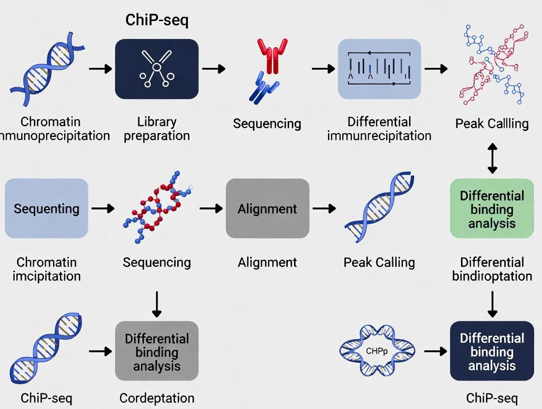
Workflow and Relationship Visualizations
Diagram 1: From Cells to Data - ChIP-seq Experimental & Analysis Workflow
Diagram 2: Key Biological Questions Answered by ChIP-seq
Robust Chromatin Immunoprecipitation followed by sequencing (ChIP-seq) is foundational for epigenetics and transcriptional regulation studies in drug development and basic research. The validity of the resulting data hinges on three pillars: high-specificity antibodies, appropriate controls (Input and IgG), and biological replicates. Omitting or mishandling any component introduces confounding variables, leading to irreproducible or false-positive findings.
The Role of Antibodies
The antibody is the core targeting agent. Its quality directly determines signal-to-noise ratio.
- Primary Antibody: Must be validated for ChIP (ChIP-seq grade). Key metrics include specificity (single band on western blot), affinity, and lot-to-lot consistency.
- Key Consideration: Polyclonal vs. Monoclonal. Polyclonals offer signal amplification but risk batch variability. Monoclonals provide superior specificity but may have lower affinity for some epitopes in fixed chromatin.
The Criticality of Controls
Controls are non-negotiable for accurate peak calling and interpretation.
- Input DNA Control: Sheared, non-immunoprecipitated chromatin. Accounts for genomic regions prone to non-specific enrichment (e.g., open chromatin, high GC content).
- IgG Isotype Control: Immunoprecipitation with a non-specific antibody. Identifies background noise from non-specific antibody binding or protein A/G bead interactions.
The Necessity of Replicates
Replicates address biological variability and statistical power.
- Biological Replicates: Independent biological samples (e.g., cells from different passages/treatments). Essential for assessing consistency and performing statistically rigorous differential binding analysis.
- Technical Replicates: Multiple library preparations from the same IP'd DNA. Primarily assess library construction variability.
Table 1: Summary of Minimum Experimental Design Requirements for Publication-Quality ChIP-seq
| Component | Minimum Recommended Number | Purpose | Consequence of Omission |
|---|---|---|---|
| Specific Antibody | 1 per target | Target-specific enrichment | No experiment; false negatives |
| Input Control | 1 per cell type/condition | Background genomic profile reference | Inability to distinguish true peaks from artifacts |
| IgG Control | 1 per experiment | Background IP noise reference | High false positive rate in peak calling |
| Biological Replicates | 2 (minimum), 3+ (ideal) | Account for biological variation; enable statistics | Findings are not generalizable; unreliable p-values |
| Technical Replicates | Optional | Assess technical noise | Cannot parse technical from biological variation |
Detailed Protocols
Protocol: Input DNA Preparation
This protocol runs in parallel with the main ChIP procedure.
Materials:
- Sheared, cross-linked chromatin (from main ChIP protocol)
- 5M NaCl
- RNase A (10 mg/ml)
- Proteinase K (20 mg/ml)
- Phenol:Chloroform:Isoamyl Alcohol (25:24:1)
- Glycogen (20 mg/ml)
- 100% and 70% Ethanol
- TE Buffer (10 mM Tris-HCl, 1 mM EDTA, pH 8.0)
Method:
- Decrosslinking: Take 10% (typical) of the total sheared chromatin volume and place in a fresh tube. Add NaCl to a final concentration of 200 mM.
- Incubate: Heat at 65°C for 4-6 hours (or overnight) to reverse crosslinks.
- RNA Digestion: Add 1 µl of RNase A. Incubate at 37°C for 30 min.
- Protein Digestion: Add 2 µl of Proteinase K. Incubate at 55°C for 1-2 hours.
- DNA Purification: a. Extract once with an equal volume of Phenol:Chloroform:Isoamyl Alcohol. Centrifuge. b. Transfer aqueous phase to a new tube. Add 1 µl glycogen, 0.1 volumes 3M NaOAc (pH 5.2), and 2.5 volumes 100% ethanol. c. Precipitate at -80°C for 1 hour or -20°C overnight. d. Pellet DNA by centrifugation at max speed for 15 min at 4°C. e. Wash pellet with 1 ml ice-cold 70% ethanol. Centrifuge for 5 min. f. Air-dry pellet and resuspend in 50 µl TE Buffer or nuclease-free water.
- Quantification: Measure DNA concentration using a fluorometric assay (e.g., Qubit). Proceed to library preparation.
Protocol: IgG Control Immunoprecipitation
Perform this alongside the target-specific IP.
Materials:
- Sheared, cross-linked chromatin
- Species-matched Normal IgG (e.g., Rabbit IgG for a rabbit primary antibody)
- Protein A/G Magnetic Beads
- ChIP Lysis/Wash Buffers (as per main protocol)
- Elution Buffer (1% SDS, 100 mM NaHCO3)
Method:
- Bead Preparation: Prepare Protein A/G beads as per main protocol.
- Set-Up Reaction: Use the same amount of chromatin as for the specific IP. Add an equivalent mass (µg) of Normal IgG as used for the specific antibody.
- Immunoprecipitation: Follow the identical incubation, wash, and elution steps as the main ChIP protocol.
- Decrosslinking & Purification: Process the eluate alongside the specific IP samples (as described in Section 2.1, steps 1-6).
Diagrams
ChIP-seq Experimental Workflow with Controls
How Controls Are Used in Peak Calling
The Scientist's Toolkit
Table 2: Research Reagent Solutions for Robust ChIP-seq
| Item | Function & Importance | Example/Notes |
|---|---|---|
| ChIP-seq Grade Antibody | Highly specific antibody validated for use in ChIP. The single most critical reagent. | Suppliers: Cell Signaling Technology (CST), Abcam, Diagenode. Check for cited ChIP-seq data. |
| Species-Matched Normal IgG | Isotype control for non-specific binding during IP. Essential for background definition. | Must match host species (e.g., Rabbit IgG for rabbit primary). |
| Protein A/G Magnetic Beads | Efficient capture of antibody-antigen complexes. Magnetic beads simplify washing. | Choose bead type (A, G, or A/G) based on antibody species and subclass for optimal binding. |
| Crosslinking Reagent | Stabilizes protein-DNA interactions. Choice affects epitope availability and resolution. | Formaldehyde (standard); DSG/Formaldehyde for distant epitopes. |
| Chromatin Shearing System | Fragments chromatin to optimal size (200-500 bp). Consistency is key for resolution. | Sonication (Covaris recommended) or enzymatic (MNase). |
| DNA Clean/Concentrator Kit | For purifying DNA after decrosslinking. Efficient recovery of low-concentration samples. | Zymo Research kits are widely used. |
| High-Sensitivity DNA Assay | Accurately quantifies low amounts of purified ChIP DNA prior to library prep. | Qubit dsDNA HS Assay (fluorometric). Avoid spectrophotometry. |
| Library Prep Kit for Low Input | Converts picogram amounts of ChIP DNA into sequencer-compatible libraries. | Illumina, NEB, or Takara kits validated for low-input/ChIP-seq. |
| SPRI Beads | Size-selects and purifies DNA fragments (e.g., post-ligation, post-PCR). Replaces gels. | AMPure/SPRIselect beads. |
Within a ChIP-seq data analysis workflow, raw sequencing data is progressively transformed, interpreted, and annotated through a series of standardized file formats. Each format encapsulates specific information, from sequence reads to aligned genomic coordinates and finally to identified protein-DNA binding sites. This primer details the structure, application, and interconversion of four cornerstone file types in the ChIP-seq pipeline.
File Format Specifications and Quantitative Comparison
Table 1: Core File Format Specifications in ChIP-seq Analysis
| Format | Primary Use | Standard Columns/Fields | Key Information Encoded | Binary/Text | Size Relative |
|---|---|---|---|---|---|
| FASTQ | Raw sequencing output | 4 lines per record: 1) Read ID, 2) Sequence, 3) Separator (+), 4) Quality scores | Nucleotide sequence, machine identifier, per-base sequencing quality (Phred scores) | Text | Very Large (GBs) |
| BAM | Aligned sequencing reads | Predefined SAM fields (e.g., QNAME, FLAG, RNAME, POS, MAPQ, CIGAR, RNEXT, PNEXT, TLEN, SEQ, QUAL) | Aligned genomic coordinates, mapping quality, insert size, mate pair info, sequence, quality. | Binary (compressed) | Large (10-30% of FASTQ) |
| BED | Genomic intervals & annotations | Minimum 3: 1) chrom, 2) chromStart, 3) chromEnd. Up to 12 standard fields. | Genomic regions (0-start, half-open), name, score, strand, thick/display coordinates, RGB color. | Text | Very Small (KBs-MBs) |
| NarrowPeak | ChIP-seq peaks (transcription factors) | 10 columns: BED6 + 4 extras (signalValue, pValue, qValue, summit). | Peak location, statistical significance (p/q-value), enrichment fold-change, summit offset. | Text | Small (MBs) |
| BroadPeak | ChIP-seq broad marks (histones) | 9 columns: BED6 + 3 extras (signalValue, pValue, qValue). | Broad enrichment region, statistical significance, signal strength. | Text | Small (MBs) |
Table 2: Key Software for Format Processing in ChIP-seq
| Software/Tool | Primary Function | Key Input Format | Key Output Format |
|---|---|---|---|
| bwa-mem / Bowtie2 | Read alignment | FASTQ | SAM/BAM |
| samtools | SAM/BAM manipulation, sorting, indexing | SAM/BAM | BAM, CRAM, indices |
| MACS2 | Peak calling | BAM | NarrowPeak, BroadPeak |
| bedtools | Interval arithmetic, intersections | BED, BAM, GFF | BED, BAM |
| SEACR | Peak calling (sparse data) | BEDGRAPH | BED (NarrowPeak-like) |
Detailed Methodologies and Protocols
Protocol 1: From FASTQ to Aligned BAM (Read Alignment) Objective: Map sequencing reads to a reference genome.
- Quality Control: Use
fastqcon raw FASTQ files. Trim adapters and low-quality bases withtrim_galoreorcutadapt. - Index Reference Genome: Generate an index for your reference genome (e.g., hg38) using the aligner (e.g.,
bowtie2-build genome.fa genome_index). - Alignment: Execute alignment. Example with Bowtie2:
- SAM to BAM Conversion: Convert SAM to compressed BAM, sort, and index using
samtools:
Protocol 2: From BAM to Peak Calls using MACS2 Objective: Identify statistically significant regions of enrichment (peaks).
- Input Preparation: Ensure you have a sorted, indexed BAM file for the ChIP sample and a matched control (Input/IgG) sample.
- Narrow Peak Calling (for TFs):
- Broad Peak Calling (for histone marks):
- Output: Primary outputs are
*_peaks.narrowPeakor*_peaks.broadPeakfiles, and*_peaks.xlscontaining detailed metrics.
Protocol 3: Peak Annotation and Visualization with BED Tools Objective: Determine genomic features nearest to peaks and create visualization files.
- Annotate Peaks: Use tools like
ChIPseeker(R/Bioconductor) orannotatePeaks.pl(HOMER) to associate peaks with nearby genes, TSS distances, etc. - Generate Coverage Tracks: Create a normalized BigWig file for genome browser visualization.
- Intersect with Genomic Features: Use
bedtools intersectto find peaks overlapping promoters, enhancers, etc.
Visual Workflows
ChIP-seq Data Analysis Workflow
(Diagram Title: ChIP-seq File Format Transformation Pipeline)
Logical Relationship of File Formats
(Diagram Title: File Format Relationships in ChIP-seq)
The Scientist's Toolkit: Essential Research Reagents & Solutions
Table 3: Key Reagents and Computational Tools for ChIP-seq Experiments
| Item/Tool | Function/Application | Example/Note |
|---|---|---|
| Crosslinking Agent | Fixes protein-DNA interactions | Formaldehyde (1% final concentration). |
| ChIP-grade Antibody | Immunoprecipitates target protein/protein modification. | Validated, high-specificity antibody (e.g., anti-H3K27ac, anti-CTCF). |
| Protein A/G Magnetic Beads | Captures antibody-target complexes. | Beads with low non-specific DNA binding. |
| DNA Purification Kit | Recovers immunoprecipitated DNA after reversal of crosslinks. | Column-based or SPRI bead-based clean-up. |
| Sequencing Library Prep Kit | Prepares ChIP DNA for high-throughput sequencing. | Kits optimized for low-input DNA (e.g., ThruPLEX). |
| Alignment Software (Bowtie2/BWA) | Maps reads to reference genome. | Requires reference genome index (e.g., hg38). |
| Peak Calling Software (MACS2) | Identifies statistically enriched genomic regions. | Requires paired ChIP and control BAM files. |
| Genome Browser (IGV/UCSC) | Visualizes alignment (BAM) and enrichment (BigWig, BED) tracks. | Critical for quality assessment and result interpretation. |
Within a comprehensive ChIP-seq data analysis thesis, the initial quality control (QC) of raw sequencing reads is a critical, non-negotiable step. The quality of downstream analyses—peak calling, motif discovery, and differential binding assessment—is fundamentally constrained by the quality of the input data. This protocol details the application of FastQC for individual assessment and MultiQC for aggregated reporting, forming the essential first chapter in a robust, reproducible ChIP-seq workflow.
Research Reagent & Software Toolkit
| Item | Function & Relevance |
|---|---|
| Raw FASTQ Files | The primary input containing sequence reads and per-base quality scores from the sequencer (e.g., Illumina). |
| FastQC (v0.12.1+) | A Java tool providing a modular set of analyses which give a quick impression of potential problems in raw read data. |
| MultiQC (v1.15+) | A Python tool that aggregates results from multiple FastQC runs (and other tools) into a single, interactive HTML report. |
| Command-line Environment | Linux/Unix terminal or Windows Subsystem for Linux (WSL) for executing bioinformatics tools. |
| Sufficient Computational Resources | Adequate RAM (≥4GB) and storage for processing large sequencing files. |
Quantitative Metrics Assessed by FastQC
FastQC evaluates several key metrics, summarized below with their pass/warn/fail status implications.
Table 1: Core FastQC Modules and Interpretation Guidelines
| Module | Metric Assessed | Typical "Good" Outcome (Pass) | Potential "Fail" Cause in ChIP-seq |
|---|---|---|---|
| Per Base Sequence Quality | Phred scores across all bases. | Quality scores >28 across the read. | Drop in quality at read ends; indicative of sequencing chemistry issues. |
| Per Sequence Quality Scores | Average quality per read. | A sharp peak in the high-quality region. | A broad or low-quality peak suggests a subset of poor-quality reads. |
| Per Base Sequence Content | Proportion of A/T/C/G per position. | Flat lines, after considering first ~10 bases. | Non-flat profiles after position ~12 may indicate overrepresented contaminants or adapter presence. |
| Adapter Content | Percentage of reads containing adapter sequences. | Near 0% adapter presence. | High levels signal required adapter trimming prior to alignment. |
| Overrepresented Sequences | Reads or kmers appearing disproportionately. | None significantly overrepresented. | Common in ChIP-seq: PCR duplicates, adapter dimers, or dominant genomic regions (e.g., rRNA). |
| Sequence Duplication Levels | Proportion of identically duplicated reads. | High diversity (low duplication) in a diverse library. | Note: ChIP-seq libraries expectedly have high duplication due to enriched regions; this module often "fails" correctly. |
Detailed Experimental Protocol
Protocol 4.1: Initial FastQC Analysis on Single or Paired-end Reads
Objective: To generate a quality report for a single FASTQ file or a pair of files (R1, R2).
Software Installation:
Run FastQC:
-o: Specifies output directory.-t: Number of threads to use for parallel processing.
Output Interpretation:
- Navigate to the output directory and open the
sample_R1_fastqc.htmlfile in a web browser. - Systematically review each module (Table 1), paying particular attention to "Adapter Content" and "Per Base Sequence Quality". Note any "Fail" flags.
- Navigate to the output directory and open the
Protocol 4.2: Aggregate Reports with MultiQC for a Full Experiment
Objective: To compile FastQC results from multiple samples into a single report for cross-sample comparison.
Run MultiQC:
- MultiQC automatically searches the current directory (
.) for recognizable log files.
- MultiQC automatically searches the current directory (
Output Interpretation:
- Open the generated
multiqc_report.html. - Use the "General Statistics" table at the top for a rapid overview of all samples.
- Click on individual plots (e.g., "Mean Quality Scores") to interactively compare all samples. This is critical for identifying outlier datasets in a batch.
- Open the generated
Visualization of the QC Workflow
Title: ChIP-seq Raw Read Quality Control Decision Workflow
Critical Interpretation for ChIP-seq Data
- High Duplication Levels: Unlike RNA-seq, this is expected in ChIP-seq due to the enrichment of specific genomic regions. Do not use it as a sole criterion for filtering unless linked to PCR artifacts.
- Sequence Content Bias: A skewed GC content profile may reflect the true biology of protein-binding regions (e.g., TF binding to GC-rich promoters). Compare to input/DNAse-seq controls.
- Adapter Contamination: This is a major, actionable finding. Adapters must be trimmed (using tools like
cutadaptorTrimmomatic) before alignment to prevent mapping failures.
Table 2: Actionable Responses to Common FastQC Outcomes in ChIP-seq
| Finding | Typical Module Flag | Recommended Action |
|---|---|---|
| Low quality at read ends | Per Base Quality (Fail/Warn) | Implement gentle quality trimming or soft-clipping during alignment. |
| Significant adapter contamination | Adapter Content (Fail) | Perform strict adapter trimming prior to alignment. |
| Overall low sequence quality | Per Sequence Quality (Fail) | Contact sequencing facility; consider discarding the library. |
| High duplication rate | Sequence Duplication (Fail) | Interpret in context. Proceed, but mark duplicates post-alignment. |
| Overrepresented sequences | Overrepresented Seqs (Fail) | Identify sequence; if adapter, trim; if PCR dimer, consider filtering. |
This protocol establishes the foundational QC checkpoint. The aggregated MultiQC report should be included as a figure in the thesis materials chapter, with outliers noted and remediation steps justified. Only data passing these thresholds should advance to the next stage of the ChIP-seq workflow: alignment to a reference genome.
Within the comprehensive workflow of a ChIP-seq data analysis thesis, the alignment of sequencing reads to a reference genome is a critical step that directly influences all subsequent interpretations. This step involves computationally mapping millions of short DNA fragments (reads) generated by the sequencer to their most likely locations in a known reference genome. Accurate alignment is paramount for correctly identifying protein-DNA interaction sites in ChIP-seq experiments. This protocol details the application of two industry-standard alignment tools, Bowtie 2 and BWA, and defines the key metrics used to evaluate mapping performance.
The choice of aligner involves trade-offs between speed, sensitivity, and memory usage. The following table summarizes the core characteristics of Bowtie 2 and BWA-MEM, the most widely used algorithm in the BWA suite for longer reads typical of modern sequencing platforms.
Table 1: Comparison of Bowtie 2 and BWA-MEM Aligners
| Feature | Bowtie 2 | BWA-MEM |
|---|---|---|
| Primary Algorithm | Burrows-Wheeler Transform (BWT) with FM-index | Burrows-Wheeler Transform (BWT) with FM-index |
| Best Read Length | 50 bp - 1000+ bp (optimal for 50-100bp) | 70 bp - 1 Mbp+ (optimal for 70-100bp+) |
| Speed | Very Fast | Fast |
| Memory Usage | Moderate (~3.5 GB for human genome) | Moderate (~3.5 GB for human genome) |
| Gapped Alignment | Yes (local alignment) | Yes (local alignment) |
| Split Read Alignment | Limited | Excellent (for SVs, long indels) |
| Paired-End Handling | Excellent | Excellent |
| Typical ChIP-seq Use | Excellent for transcription factor studies (shorter reads) | Excellent for histone marks (longer reads, handles indels better) |
| Key Strength | Speed and accuracy for standard alignments | Versatility, handling of longer reads & structural variants |
| Common Output Format | SAM/BAM | SAM/BAM |
Key Mapping Metrics for Quality Assessment
After alignment, it is crucial to assess the quality of the mapping. The following metrics, often reported by tools like samtools flagstat and samtools stats, should be examined.
Table 2: Essential Post-Alignment Mapping Metrics
| Metric | Definition | Ideal Target (ChIP-seq) | Interpretation |
|---|---|---|---|
| Total Reads | Total number of reads in the FASTQ file. | N/A | Baseline count. |
| Overall Alignment Rate | Percentage of total reads that aligned to the reference. | > 70-90% (genome-dependent) | Low rates may indicate contamination or poor-quality reads. |
| Uniquely Mapped Reads | Percentage of reads mapping to a single, unique location in the genome. | High (typically >70-80% of mapped) | Critical for ChIP-seq. Multi-mapping reads are often discarded. |
| Multi-mapping Reads | Reads that align to multiple genomic loci with equal quality. | As low as possible | Can confound peak calling; often filtered out. |
| Reads Mapped in Proper Pairs | For paired-end data, the percentage where both mates align correctly relative to the expected insert size and orientation. | > 90% of mapped paired reads | Indicates high-quality library prep and alignment. |
| Duplicate Rate | Percentage of reads that are PCR duplicates. | < 20-30% (library dependent) | High rates reduce effective sequencing depth. Measured after alignment. |
Detailed Experimental Protocols
Protocol 4.1: Indexing the Reference Genome
- Objective: Create a searchable index of the reference genome to enable rapid alignment.
Materials:
- Reference genome FASTA file (e.g.,
hg38.fa). - Bowtie 2 or BWA software installed.
- High-performance computing server with adequate memory.
- Reference genome FASTA file (e.g.,
Methodology for Bowtie 2:
- This generates a set of
.bt2files.
- This generates a set of
Methodology for BWA:
- This generates files with extensions like
.amb,.ann,.bwt,.pac,.sa.
- This generates files with extensions like
Protocol 4.2: Aligning Single-End ChIP-seq Reads
- Objective: Map single-end sequencing reads to the reference genome.
Materials: Indexed reference genome, FASTQ file of reads (
sample.fastq).Methodology for Bowtie 2:
Methodology for BWA-MEM:
Protocol 4.3: Aligning Paired-End ChIP-seq Reads
- Objective: Map paired-end reads, preserving mate-pair information.
Materials: Indexed reference genome, paired FASTQ files (
sample_R1.fastq,sample_R2.fastq).Methodology for Bowtie 2:
Methodology for BWA-MEM:
Protocol 4.4: Post-Alignment Processing and Metric Calculation
- Objective: Convert SAM to BAM, sort, and calculate mapping statistics.
Materials: SAM file from alignment,
samtoolssoftware.Methodology:
Visualization of the Alignment Workflow in ChIP-seq Analysis
Diagram 1: Read Alignment and QC Workflow
The Scientist's Toolkit: Essential Research Reagents & Materials
Table 3: Key Resources for Read Alignment in ChIP-seq Analysis
| Item | Function in the Alignment Step |
|---|---|
| Reference Genome FASTA File | The nucleotide sequence of the target organism (e.g., GRCh38 for human) against which reads are mapped. |
| Alignment Software (Bowtie2/BWA) | The core algorithm that performs the sequence search and mapping against the indexed genome. |
| High-Performance Computing (HPC) Cluster | Provides the necessary CPU power and memory to run alignment jobs efficiently on large datasets. |
| SAM/BAM Tools (samtools, picard) | Software suites for manipulating, sorting, indexing, and assessing aligned read files. |
| Quality Control Software (FastQC, MultiQC) | Used before and after alignment to assess read quality and summarize metrics across samples. |
| Genome Index Files | The pre-processed, searchable database generated from the reference FASTA file by the aligner. |
| Sequencing Adapter Sequences | Known adapter sequences used during library prep, which may be trimmed pre-alignment to improve mapping rates. |
Application Notes
Within the comprehensive ChIP-seq data analysis workflow, the initial visualization of processed sequencing data is a critical step for quality assessment and hypothesis generation. After alignment and the generation of continuous coverage tracks (BigWig files), researchers must load these files into genome browsers to visually inspect signal distribution, peak enrichment, and background noise across the genome. This protocol details the methodology for loading BigWig files into two predominant genome browsers: the Integrative Genomics Viewer (IGV) and the UCSC Genome Browser. Effective visualization at this stage enables researchers to confirm experimental success, identify potential artifacts, and guide subsequent quantitative analyses like peak calling.
Experimental Protocols
Protocol 1: Loading BigWig Files into the Integrative Genomics Viewer (IGV)
Principle: IGV is a high-performance desktop application that supports interactive exploration of large genomic datasets. It is ideal for visualizing ChIP-seq signal tracks against a reference genome and annotated features.
Materials:
- Computer with IGV installed (Download from: https://software.broadinstitute.org/software/igv/)
- Processed BigWig file(s) from ChIP-seq analysis (generated via tools like
bamCoveragefrom deepTools). - (Optional) Reference genome index files and annotation files (e.g., BED, GTF).
Methodology:
- Launch and Genome Selection: Start IGV. From the drop-down menu at the top, select the appropriate reference genome (e.g., "Human hg38") that matches your data's alignment.
- Data Loading:
- Navigate to
File>Load from File...(or use the shortcutCtrl+L/Cmd+L). - Browse and select your local BigWig file(s). Multiple files can be loaded simultaneously (e.g., treatment and control).
- Navigate to
- Track Configuration: Once loaded, tracks appear in the visualization panel. Right-click on a track to adjust:
- Data Range: Set
Autoscale,Clamp Values, or a manual range to optimize signal contrast. - Color: Change the display color for clear distinction between tracks.
- View as: Ensure it is set to "Continuous" mode.
- Data Range: Set
- Navigation: Enter a genomic locus (e.g., gene name, coordinates like
chr1:50,000,000-50,100,000) in the search box to navigate. - Visual Inspection: Zoom and pan to assess signal enrichment at known binding sites, promoter regions, and globally across chromosomes.
Protocol 2: Loading BigWig Files into the UCSC Genome Browser
Principle: The UCSC Genome Browser is a web-based tool for viewing genomic data in a richly annotated, publicly shared context. It is optimal for comparing your data with a vast array of public annotation tracks.
Materials:
- Internet-connected computer.
- BigWig file(s). For public sharing, files must be hosted on a public web-accessible server (e.g., institutional server, GitHub, or cloud storage). For private viewing, use the "Custom Track" feature with local files or a signed URL.
- UCSC Genome Browser session link (if saving/loading a session).
Methodology:
- Access Browser: Navigate to https://genome.ucsc.edu.
- Open Genome Browser: Click the "Genomes" or "Genome Browser" button.
- Set Genome and Assembly: Use the "genome" and "assembly" drop-down menus to select the correct reference (e.g., "Human" and "Dec. 2013 (GRCh38/hg38)").
- Load Custom BigWig Track:
- Click "add custom tracks" on the home page, or navigate to the "My Data" > "Custom Tracks" tab after entering the Browser.
- In the "Paste URLs or data" box, you have two options:
- Option A (Remote File): Provide the direct, public HTTP/HTTPS URL to your BigWig file (one per line).
- Option B (Local File): Use the "Choose File" button to upload a BigWig file directly from your computer (size limits apply).
- Click "Submit".
- Configure Track Settings: After submission, you will be directed to the "Manage Custom Tracks" page. Click the track name to configure display parameters such as visibility, color, scaling, and priority in the stack. Save settings.
- View and Share: Navigate to a genomic region. Your track(s) will display alongside public annotation tracks. You can save the entire configuration as a "Session" to generate a shareable link for collaborators.
Data Presentation
Table 1: Comparison of BigWig Loading in IGV vs. UCSC Genome Browser
| Feature | IGV (Desktop) | UCSC Genome Browser (Web) |
|---|---|---|
| Primary Use Case | Interactive, rapid exploration of local data; ideal for analysis. | Publication-quality views & comparison with vast public datasets. |
| Data Source | Directly from local filesystem or network drive. | Requires files to be web-accessible via URL or uploaded. |
| Speed for Large Data | Very fast; loads indexed data on-demand. | Can be slower, dependent on server speed and internet connection. |
| Collaboration | Requires file sharing; sessions can be saved and shared. | Excellent; sessions and custom track URLs are easily shareable. |
| Annotation Context | Must load custom annotation files; limited built-in public tracks. | Extensive built-in public annotation database (genes, ENCODE, etc.). |
| Ideal Workflow Stage | Initial QC, iterative analysis during processing. | Final visualization, publication figure generation, data sharing. |
Visualization: Workflow Diagram
Diagram Title: BigWig Visualization Pathway in ChIP-seq Workflow
The Scientist's Toolkit
Table 2: Essential Research Reagent Solutions for BigWig Visualization
| Item | Function in Visualization |
|---|---|
| BigWig File | Binary, indexed format storing continuous-valued genomic data (e.g., read coverage scores). Essential input for browsers. |
| IGV Desktop Application | High-performance visualization software for interactive exploration of genomic data from local storage. |
| UCSC Genome Browser | Web-based platform for viewing genomic data in a public annotation context and generating shareable sessions. |
| Public Data Hub/Server | A web-accessible server (e.g., AWS S3, institutional HTTP) to host BigWig files for UCSC Browser loading via URL. |
| Genome Annotation File (GTF/BED) | Provides gene model context in IGV. Helps orient signal enrichment relative to known genomic features. |
| Track Hub Configuration Files | (Advanced) Text files (hub.txt, genomes.txt, trackDb.txt) to organize and display multiple tracks as a collection on UCSC. |
The Analytical Pipeline: Peak Calling, Annotation, and Advanced Functional Analysis
Within a comprehensive ChIP-seq data analysis workflow, the peak calling step is critical for identifying genomic regions where a protein of interest (e.g., transcription factor, histone modification) binds or resides. This note details the application and protocols for three seminal algorithms—MACS2, HOMER, and SICER—which represent core methodological approaches to this problem.
Algorithmic Principles and Quantitative Comparison
Core Methodologies
- MACS2 (Model-based Analysis of ChIP-seq 2): Employs a dynamic Poisson distribution to model the shift size of sequenced tags, building a local lambda parameter for background estimation to identify significant peaks with high sensitivity, especially for transcription factors.
- HOMER (Hypergeometric Optimization of Motif EnRichment): Utilizes a position-specific scoring matrix to find peaks and is uniquely integrated with powerful de novo and known motif discovery tools, making it a suite for both peak calling and downstream analysis.
- SICER (Spatial Clustering for Identification of ChIP-Enriched Regions): Designed specifically for diffuse histone marks, it uses a clustering approach to identify broad domains of enrichment by accounting for spatial distribution of reads, reducing false positives from random noise.
The following table summarizes key characteristics and typical performance metrics based on benchmark studies.
Table 1: Comparison of Peak Calling Algorithms
| Feature | MACS2 | HOMER | SICER |
|---|---|---|---|
| Primary Strength | Sharp peak resolution (TFs) | Integrated motif analysis | Broad peak identification (histones) |
| Statistical Model | Dynamic Poisson, local background | Binomial, FDR control | Clustering-based, Poisson & FDR |
| Key Input Requirement | Treatment and control (e.g., Input/IgG) BAM files | Treatment and control BAM files or tag directories | Treatment and control BAM files |
| Typical Sensitivity | High for narrow peaks | Moderate, highly motif-correlated | High for broad, diffuse regions |
| Typical Runtime (Speed) | Fast | Moderate (slower with motif finding) | Slow (due to clustering) |
| Critical Parameter | --qvalue (or -p), --broad |
-F (fold change), -size |
-w (window size), -g (gap size) |
Detailed Experimental Protocols
Protocol 1: Peak Calling with MACS2
Application: Standard peak calling for transcription factor ChIP-seq data.
- Prerequisite: Aligned reads in BAM format for both ChIP (
chip.bam) and control/input (input.bam) samples. - Command for Narrow Peaks:
- Command for Broad Histone Marks:
Protocol 2: Peak Calling & Motif Discovery with HOMER
Application: Peak calling with immediate integrated motif analysis.
- Create Tag Directories:
Run Peak Calling:
-style: Peak finding style (factorfor TFs,histonefor broad marks).-o: Output file.-i: Input control tag directory.
- Run De Novo Motif Discovery:
Protocol 3: Identifying Broad Domains with SICER
Application: Detection of broad enriched regions for histone modifications like H3K27me3.
- Convert BAM to BED:
Run SICER with Recommended Parameters:
- Arguments: Input directory, treatment file, control file, output directory, species, redundancy threshold, window size, gap size, FDR, FDR for broad regions.
Visualization of ChIP-seq Analysis Workflow
ChIP-seq Data Analysis Core Workflow
The Scientist's Toolkit: Key Research Reagent Solutions
Table 2: Essential Reagents & Materials for ChIP-seq Experiments
| Reagent/Material | Function in ChIP-seq Workflow |
|---|---|
| Specific Antibody | Immunoprecipitates the target protein-DNA complex. Critical for specificity and signal-to-noise. |
| Protein A/G Magnetic Beads | Efficient capture and purification of antibody-bound complexes, facilitating washing and elution. |
| Crosslinking Agent (e.g., Formaldehyde) | Fixes protein-DNA interactions in vivo prior to cell lysis and fragmentation. |
| Chromatin Shearing Reagents | Enzymatic (e.g., MNase) or sonication kits for fragmenting crosslinked chromatin to optimal size. |
| DNA Clean-up/Size Selection Kits | Purify and select library fragments post-library preparation, crucial for sequencing quality. |
| High-Fidelity PCR Master Mix | Amplifies the ChIP-enriched DNA library with minimal bias for sequencing. |
| High-Sensitivity DNA Assay Kits | Accurately quantify low-concentration ChIP and library DNA (e.g., Qubit, Bioanalyzer). |
| Sequencing Library Prep Kit | Provides all necessary enzymes and buffers for end-repair, A-tailing, and adapter ligation. |
| Indexed Sequencing Adapters | Allow multiplexing of multiple samples in a single sequencing run. |
| Control Samples (Input/IgG) | Genomic DNA control (Input) and non-specific antibody control (IgG) essential for accurate peak calling. |
Within a comprehensive ChIP-seq data analysis thesis, the selection of appropriate parameters for peak calling is a critical, yet often nuanced, step that differs significantly between transcription factor (TF) and histone mark experiments. This protocol details the rationale and methods for choosing stringency thresholds, fragment shift sizes, and statistical models, ensuring accurate biological interpretation.
Key Parameter Comparison Table
Table 1: Core Parameter Recommendations for TF vs. Histone Mark ChIP-seq
| Parameter | Transcription Factor (TF) ChIP-seq | Histone Mark ChIP-seq (e.g., H3K4me3, H3K27ac) | Histone Mark ChIP-seq (Broad, e.g., H3K9me3, H3K36me3) |
|---|---|---|---|
| Expected Peak Profile | Sharp, narrow (50-300 bp) | Sharp, narrow to broad (500-2000 bp) | Very broad (≥5 kb) |
| Recommended Shift Size | Fragment length/2 (e.g., 75-150 bp). Estimate from cross-correlation. | Fragment length/2 (e.g., 100-200 bp). | Often no shifting or a small shift; broad enrichment modeling is more critical. |
| Primary Peak Calling Model | Fixed-size peak models (e.g., in MACS2). Assumes a fixed window size. | Variable-width or fixed-size models. MACS2 --broad flag is common. |
Broad domain detection algorithms (e.g., SICER2, BroadPeak in MACS2, RSEG). |
| Stringency (p-value/FDR) | Typically more stringent (e.g., p-value 1e-5 to 1e-10; FDR 0.1-1%). Fewer, high-confidence peaks. | Moderate stringency (e.g., p-value 1e-3 to 1e-5; FDR 1-5%). Balances sensitivity/specificity. | Less stringent (e.g., FDR 5-10%). Required to capture diffuse enrichment regions. |
| Key Control | Input DNA or IgG. Critical for modeling background. | Input DNA. Essential for broad mark analysis. | Input DNA. Vital due to low signal-to-noise in broad domains. |
| Typical Peak Count | Low (1,000 - 50,000) | Moderate (10,000 - 100,000) | Low count of very large regions (1,000 - 20,000 domains) |
Experimental Protocols
Protocol 3.1: Empirical Determination of Shift Size using Cross-Correlation
Purpose: To calculate the optimal fragment shift size for aligning forward and reverse reads prior to peak calling.
Materials:
- Aligned BAM file (ChIP-seq sample).
- Computing environment with deepTools or phantompeakqualtools installed.
Procedure:
- Subsample Reads: Use
samtools view -sto subsample 1-5 million reads from your BAM file to reduce computation time. - Calculate Cross-Correlation: Run
plotFingerprintfrom deepTools orspp.Rfrom phantompeakqualtools.- deepTools command example:
- deepTools command example:
- Interpret Output: The cross-correlation plot shows the correlation between forward and reverse strands at different shift values. The Strand Shift at the maximum correlation (the "phantom peak") represents the recommended fragment length for shifting (d). The true peak shift size is d/2.
- Apply Parameter: Use the calculated
d/2value as the--shiftor--extsizeparameter in your peak caller (consult tool documentation).
Protocol 3.2: Peak Calling for Transcription Factors using MACS2
Purpose: To identify narrow, high-confidence binding sites.
Materials:
- Treatment BAM file (TF ChIP-seq).
- Control BAM file (Input DNA).
- MACS2 software.
Procedure:
- Base Command:
- Alternative (Model Building): If fragment size is unknown, omit
--nomodel,--shift, and--extsize. MACS2 will build a model. - Output:
TF_Experiment_peaks.narrowPeakcontains called peaks. UseTF_Experiment_peaks.xlsfor summary statistics.
Protocol 3.3: Peak Calling for Histone Marks using MACS2 Broad Mode
Purpose: To identify broad regions of enrichment.
Materials:
- Treatment BAM file (Histone Mark ChIP-seq).
- Control BAM file (Input DNA).
- MACS2 software.
Procedure:
- Base Command:
- Adjust Stringency: Modify
-q(for narrow regions) and--broad-cutoffbased on mark specificity. - Output: Key files are
Histone_Mark_Experiment_peaks.broadPeakandHistone_Mark_Experiment_peaks.gappedPeak.
Protocol 3.4: Parameter Optimization via IDR for TFs
Purpose: To select an optimal p-value threshold by assessing reproducibility between replicates.
Materials:
- Peak files from two biological replicates, called at varying p-value thresholds (e.g., 1e-3, 1e-5, 1e-7).
- IDR (Irreproducible Discovery Rate) software package.
Procedure:
- Call Peaks at Multiple Thresholds: Run MACS2 on each replicate with relaxed
-pvalues (e.g., 0.01, 0.001). - Run IDR: Compare the ranked peak lists from the two replicates.
- Analyze Output: The IDR output file includes a threshold (typically IDR < 0.05 or 0.1) indicating reproducible peaks. The number of peaks passing this threshold at different initial p-values guides the selection of a stringent, reproducible cutoff.
Visualizations
Diagram 1: Parameter Decision Workflow for ChIP-seq Analysis
Diagram 2: Fragment Shift Size Determination Logic
The Scientist's Toolkit
Table 2: Essential Research Reagent Solutions & Materials
| Item | Function/Description | Example/Notes |
|---|---|---|
| ChIP-Grade Antibody | Highly validated antibody specific to the target TF or histone modification. Critical for signal specificity. | For TFs: check ENCODE validation. For histones: use mod-specific antibodies (e.g., anti-H3K27ac). |
| Protein A/G Magnetic Beads | Efficient capture of antibody-protein-DNA complexes, enabling low-background washing. | Compatible with automation. Choice depends on antibody species/isotype. |
| Sonication Device | Fragments chromatin to optimal size (100-500 bp). Key for resolution. | Diagenode Bioruptor (water bath) or Covaris (focused ultrasonicator). |
| Library Prep Kit (NGS) | Prepares immunoprecipitated DNA for high-throughput sequencing. | Kits with low input compatibility (e.g., from NEB, Illumina) are essential. |
| SPRI Beads | Size selection and purification of DNA libraries; replaces gel extraction. | AMPure XP beads. Ratio determines size cutoff. |
| qPCR Primers | For positive & negative control genomic regions. Validates ChIP enrichment pre-sequencing. | Design primers for known binding sites and gene deserts. |
| High-Sensitivity DNA Assay | Accurately quantifies low-concentration ChIP DNA and libraries (e.g., Qubit, Bioanalyzer). | Fluorometric assays are superior to absorbance for low concentration. |
Within the broader ChIP-seq data analysis workflow, the step of annotating identified peaks to genomic features is critical for biological interpretation. This process assigns protein-DNA interaction sites—such as transcription factor binding or histone modification marks—to functional elements like promoters, enhancers, and gene bodies, transforming coordinate lists into actionable biological insights relevant to gene regulation studies and drug target discovery.
Key Genomic Features and Annotation Standards
Promoters
Promoters are regulatory regions immediately upstream of transcription start sites (TSSs). Standard annotation defines the promoter region as within -1 kb to +100 bp relative to the TSS, though this window can be adjusted based on biological context.
Enhancers
Enhancers are distal regulatory elements that can be located upstream, downstream, or within introns of target genes. They are often identified by specific chromatin signatures (e.g., H3K27ac, H3K4me1) and can be several kilobases from the TSS.
Gene Bodies
Gene bodies encompass the entire transcribed region from the TSS to the transcription termination site, including exons and introns. Peaks in gene bodies may be associated with elongation-related marks or regulatory elements.
Quantitative Distribution of Peaks
Table 1 presents typical peak distribution across features from a public H3K4me3 (promoter mark) and H3K36me3 (gene body mark) ChIP-seq dataset.
Table 1: Representative Peak Distribution Across Genomic Features
| Genomic Feature | H3K4me3 (%) | H3K36me3 (%) | Typical Distance from TSS (bp) |
|---|---|---|---|
| Promoter (≤ 1kb from TSS) | 65.2 | 5.1 | -1000 to +100 |
| 5' UTR | 8.7 | 12.4 | Within 5' UTR |
| 3' UTR | 3.1 | 15.3 | Within 3' UTR |
| Exon | 4.5 | 18.9 | Within exonic region |
| Intron | 12.1 | 40.7 | Within intronic region |
| Downstream (≤ 3kb) | 2.3 | 3.5 | +100 to +3000 |
| Intergenic | 4.1 | 4.1 | > 3kb from gene |
Protocol: Peak Annotation Using ChIPseeker in R
Materials and Reagents
- Computational Environment: R (version ≥4.1), Bioconductor.
- Software Packages:
ChIPseeker,GenomicFeatures,TxDb.Hsapiens.UCSC.hg38.knownGene(or species-appropriate). - Input Data: BED or narrowPeak file from peak callers (MACS2, SPP).
- Genome Annotation File: Reference transcript database (TxDb) or GTF/GFF3 file.
Method
Preparation of Annotation Database
Load Peak Data
Annotate Peaks
Summarize and Visualize Results
Protocol: Enhancer-Promoter Linkage Annotation Using GREAT
Materials and Reagents
- Tool: Genomic Regions Enrichment of Annotations Tool (GREAT) web server or local installation.
- Input Data: BED file of peaks.
- Genome Assembly: Specify correct reference (hg38, mm10, etc.).
Method
- Upload Peaks: Submit BED file to GREAT (http://great.stanford.edu).
- Configure Parameters: Select association rule (e.g., "Basal plus extension" with 5 kb upstream, 1 kb downstream, up to 1 Mb max extension). Choose relevant ontology databases.
- Execute Analysis: Run job to assign peaks to regulatory domains of genes.
- Interpret Output: Review tables linking distal peaks (potential enhancers) to target genes based on proximity rules. Extract genes associated with enhancer regions.
The Scientist's Toolkit
Table 2: Essential Research Reagent Solutions for ChIP-seq & Peak Annotation
| Item / Tool | Function in Workflow |
|---|---|
| MACS2 | Peak-calling algorithm; identifies genomic regions with significant ChIP-seq enrichment. |
| ChIPseeker (R/Bioconductor) | Annotates peaks to nearest genes, TSS, and genomic features; visualizes distributions. |
| GREAT | Assigns functional meaning to cis-regulatory regions by linking peaks to distant genes. |
| RefSeq / ENSEMBL GTF | Reference gene annotation file providing coordinates for promoters, UTRs, exons, introns. |
| BedTools | Suite for genomic arithmetic; used for intersecting peak files with feature coordinates. |
| HOMER | Performs de novo motif discovery and annotates peaks to genomic regions. |
| IGV (Integrative Genomics Viewer) | Visualizes peak tracks in genomic context alongside gene models and other annotations. |
Workflow and Relationship Diagrams
ChIP-seq Peak Annotation Workflow
Logical Decision Tree for Peak Annotation
Within the comprehensive ChIP-seq data analysis workflow, the identification of protein-binding sites (peaks) is an intermediate step. The ultimate biological interpretation is achieved by translating these genomic coordinates into insights about regulated biological processes, molecular functions, and cellular components. Pathway and Gene Ontology (GO) enrichment analysis are the cornerstone techniques for this translation. This protocol details the downstream bioinformatic procedures following peak calling, enabling researchers to connect chromatin occupancy data to mechanistic biology and potential therapeutic targets.
Core Concepts and Quantitative Data
Table 1: Common Enrichment Analysis Methods and Tools
| Method | Key Metric | Typical Input | Primary Output | Common Tools |
|---|---|---|---|---|
| Over-Representation Analysis (ORA) | P-value, Fold Enrichment, FDR | List of significant gene IDs | Enriched GO terms/Pathways | clusterProfiler, DAVID, g:Profiler, Enrichr |
| Gene Set Enrichment Analysis (GSEA) | Normalized Enrichment Score (NES), FDR | Ranked gene list (e.g., by signal) | Enriched/poorly enriched gene sets | GSEA software, clusterProfiler (GSEA) |
| Functional Class Scoring (FCS) | Pathway-level statistic | Gene-level statistics | Activated/suppressed pathways | PGSEA, GSVA |
Table 2: Typical Output Metrics from Enrichment Analysis
| Metric | Description | Interpretation Threshold |
|---|---|---|
| P-value | Probability of observing the enrichment by chance. | < 0.05 |
| False Discovery Rate (FDR) | Estimated proportion of false positives among significant results. | < 0.05 or < 0.1 |
| Fold Enrichment | Ratio of observed gene count in term to expected count. | > 1.5 or 2 |
| Gene Ratio | (# genes in input list & term) / (# genes in input list). | Context-dependent |
| Count | Number of genes from input list associated with the term. | - |
Experimental Protocols
Protocol 3.1: From ChIP-seq Peaks to Gene List for ORA
Objective: To generate a reliable gene list from peak regions for Over-Representation Analysis. Materials: BED file of significant peaks, reference genome annotation file (GTF/GFF), genomic tools (BEDTools, R/Bioconductor).
- Define Peak-Gene Association:
- Proximal Association: Assign peaks to the transcription start site (TSS) of the nearest gene within a defined window (e.g., ±1 kb to ±10 kb from TSS). This is common for promoters.
- Genebody Assignment: Assign peaks falling within the gene body (from TSS to TES).
- Use
bedtools closestor Bioconductor packages likeChIPseekerorGenomicRangesin R to perform the annotation.
- Remove Ambiguous/Non-Genic Peaks: Filter out peaks assigned to intergenic regions with no gene within the specified window, or peaks associated with multiple genes if a unique assignment is required.
- Compile Unique Gene List: Extract the unique set of gene identifiers (e.g., Entrez ID, Ensembl ID, Symbol) from the assigned peaks. This list is the input for ORA.
Protocol 3.2: Performing Over-Representation Analysis with clusterProfiler
Objective: To identify statistically over-represented GO terms and KEGG pathways.
Materials: R environment, clusterProfiler, org.Hs.eg.db (or species-specific annotation package), list of significant gene IDs.
- Setup and Input Preparation:
GO Enrichment Analysis:
KEGG Pathway Enrichment Analysis:
Result Visualization:
- Generate summary tables using
as.data.frame(ego). - Create dot plots:
dotplot(ego, showCategory=20). - Create enrichment maps:
emapplot(pairwise_termsim(ego)). - Create cnetplots to show gene-term networks:
cnetplot(ego, categorySize="pvalue", foldChange=foldChange_vector).
- Generate summary tables using
Protocol 3.3: Performing Gene Set Enrichment Analysis (GSEA)
Objective: To identify pathways where genes are concentrated at the extremes (top/bottom) of a ranked list, without applying a binary significance cutoff.
Materials: Ranked gene list (e.g., by -log10(p-value)*sign(logFC)), MSigDB gene set files (e.g., .gmt), GSEA software or clusterProfiler.
- Create a Ranked Gene List:
- For each gene, calculate a ranking metric. Common metrics include signed -log10(p-value) from differential binding analysis or the product of log2(fold change) and -log10(p-value).
- Sort genes in decreasing order by this metric.
- Run GSEA using clusterProfiler:
- Interpretation:
- A positive Normalized Enrichment Score (NES) indicates enrichment at the top of the list (e.g., upregulated/associated genes).
- A negative NES indicates enrichment at the bottom of the list (e.g., downregulated/repelled genes).
- Visualize using
gseaplot2(gsea_result, geneSetID = 1).
Visualization of Workflows and Relationships
Diagram 1: From ChIP-seq peaks to pathway enrichment analysis workflow.
Diagram 2: Relationship between pathways, GO terms, and ChIP-seq target genes.
The Scientist's Toolkit
Table 3: Key Research Reagent Solutions & Essential Materials
| Item | Function/Description | Example/Provider |
|---|---|---|
| Genome Annotation File | Provides genomic coordinates of genes, transcripts, and features. Essential for peak annotation. | ENSEMBL GTF, UCSC RefSeq GFF. |
| Gene Set Database | Curated collections of genes associated with specific pathways or functions. | MSigDB, KEGG, GO, Reactome. |
| Organism Annotation Package | Bridge between gene IDs and functional databases within analysis tools like R. | Bioconductor org.*.eg.db packages (e.g., org.Hs.eg.db). |
| Functional Analysis Software Suite | Integrated toolkit for performing and visualizing enrichment analyses. | R/Bioconductor (clusterProfiler, enrichplot, DOSE). |
| Peak Annotation Tool | Software to associate genomic peaks with nearby or overlapping genes. | ChIPseeker (R), HOMER annotatePeaks.pl, BEDTools. |
| High-Performance Computing (HPC) Resources | Necessary for handling large datasets and running complex analyses like permutation-based GSEA. | Local compute clusters or cloud computing (AWS, Google Cloud). |
Application Notes
Within the ChIP-seq data analysis workflow, motif discovery is the step that extracts biological meaning from high-confidence peak regions. Following peak calling and annotation, this process identifies over-represented DNA sequence patterns, inferring the binding motifs of the targeted transcription factor (TF) or co-factors. For researchers and drug development professionals, this reveals direct regulatory targets and potential intervention points. The primary computational challenge is distinguishing the true, often degenerate, motif from background genomic noise. Current best practices involve using multiple discovery algorithms on stringent peak sets and validating motifs with external databases.
Key Quantitative Comparisons of Motif Discovery Tools
Table 1: Comparison of Major *De Novo Motif Discovery Algorithms*
| Tool | Algorithm Core | Key Strength | Optimal Use Case | Typical Runtime* |
|---|---|---|---|---|
| MEME-ChIP | Expectation Maximization, Gibbs Sampling | Integrated suite for clustering & enrichment | Diverse, large peak sets (>500) | 30-60 min |
| HOMER | Hypergeometric Optimization | Speed & integrated annotation | Any peak set size, for quick analysis | 5-15 min |
| STREME | Suffix Tree Enumeration | Sensitivity for short, weak motifs | Large datasets, divergent motifs | 10-30 min |
| DREME | Regular Expression Exhaustion | Speed for short motifs (<8 bp) | Initial, fast scan of top peaks | <5 min |
*Runtime estimated for 1000 peaks on a standard server.
Table 2: Key Database Resources for Motif Validation & Matching
| Database | Motif Count | Species Focus | Key Feature | Format |
|---|---|---|---|---|
| JASPAR | >2,000 | Eukaryotic (core) | Curated, non-redundant, open-access | PFM, PWM |
| CIS-BP | >100,000 | Metazoa & Fungi | Extensive, includes predicted motifs | PWM |
| ENCODE | >1,000 | Human, Mouse | Experimentally derived from projects | PWM |
| HOCOMOCO | ~1,000 | Human, Mouse | High-quality, cell-line specific models | PWM |
Experimental Protocols
Protocol 1: De Novo Motif Discovery Using HOMER Objective: To identify de novo motifs from a set of ChIP-seq peak regions.
- Input Preparation: Generate a peak file (
peaks.bed) and a genome file (genome.fa). Create a background file or let HOMER generate it automatically. - Command Execution: Run the
findMotifsGenome.plscript.
- Output Analysis: Review the
knownResults.txt(known motif matches) andhomerResults.html(de novo motifs). Top motifs are ranked by statistical significance (p-value). - Visualization: Use
annotatePeaks.plwith the-mflag to plot motif locations within peaks.
Protocol 2: Motif Enrichment Analysis & Validation Objective: To test if a known motif from a database is enriched in the peak set.
- Motif Selection: Obtain Position Frequency Matrix (PFM) or Position Weight Matrix (PWM) from JASPAR.
- Run FIMO (MEME Suite): Scan peaks against the motif with a significance threshold.
- Calculate Enrichment: Compare the frequency of significant motif hits in peaks vs. background genomic regions using a Fisher's exact test.
- Cross-Reference: Compare discovered motifs against CIS-BP or HOCOMOCO using TOMTOM (MEME Suite) to identify the closest known TF match.
Visualizations
Title: Motif Discovery & Validation Workflow
Title: Core Logic of Motif Discovery Algorithms
The Scientist's Toolkit
Table 3: Essential Research Reagent Solutions for Motif Discovery & Validation
| Item | Function in Motif Analysis | Example/Note |
|---|---|---|
| MEME Suite | Comprehensive toolkit for de novo discovery (MEME, DREME) and enrichment (FIMO, TOMTOM). | Command-line driven, widely accepted standard. |
| HOMER | Integrated software for motif discovery, annotation, and visualization. | Preferred for its speed and all-in-one design. |
| bedtools | Critical for manipulating BED files, extracting sequences, and generating control regions. | getfasta command extracts sequences from genome. |
| JASPAR Database | Curated library of transcription factor binding profiles for motif matching. | Primary resource for known vertebrate motifs. |
| UCSC Genome Browser | Visualizes the genomic context of peaks and candidate motifs. | Essential for integrative assessment. |
| TRANSFAC | Commercial database of TF binding sites and motifs. | Historically extensive, now requires license. |
Bioconductor Packages (e.g., PWMEnrich, MotifDb) |
R-based tools for motif enrichment and analysis within statistical programming environment. | Enables reproducible analysis pipelines. |
Within the comprehensive thesis on ChIP-seq data analysis, a critical step extends beyond peak calling to functional interpretation. Integrative analysis, correlating ChIP-seq data with RNA-seq or ATAC-seq datasets, is essential for bridging the gap between transcription factor binding or histone modification landscapes and their functional outcomes in gene regulation or chromatin accessibility. This protocol details the methodologies for performing such integrative analyses to derive mechanistic insights.
Key Applications and Quantitative Outcomes
Integrative analysis answers distinct biological questions. The table below summarizes common integrative approaches and their typical quantitative outputs.
Table 1: Integrative Analysis Approaches and Outcomes
| ChIP-seq Target | Paired Dataset | Primary Biological Question | Typical Quantitative Outcome |
|---|---|---|---|
| Transcription Factor (TF) | RNA-seq (Differential Expression) | Direct transcriptional targets of the TF. | 15-30% of differentially expressed genes have a TF peak within promoter/enhancer. |
| Histone Mark (e.g., H3K27ac) | RNA-seq | Role of active enhancers/promoters in gene expression changes. | High correlation (R ~0.6-0.8) between mark intensity at regulatory regions and gene expression. |
| Transcription Factor | ATAC-seq | How TF binding alters chromatin accessibility. | 40-60% of TF binding sites show significant change in ATAC-seq signal upon TF perturbation. |
| Histone Mark (e.g., H3K4me1) | ATAC-seq | Validation and refinement of putative regulatory elements. | >70% overlap between peaks from complementary assays defining open chromatin and regulatory marks. |
Detailed Experimental Protocols
Protocol 1: Correlation of TF ChIP-seq with Differential RNA-seq Data
Objective: Identify direct target genes of a transcription factor. Steps:
- Data Generation: Perform TF ChIP-seq and RNA-seq (control vs. TF knockout/overexpression) in biological replicates.
- ChIP-seq Analysis: Call significant peaks (e.g., using MACS2). Annotate peaks to the nearest transcription start site (TSS) or defined regulatory regions (e.g., using HOMER or ChIPseeker).
- RNA-seq Analysis: Identify differentially expressed genes (DEGs) (e.g., using DESeq2 or edgeR; adj. p-value < 0.05, |log2FC| > 1).
- Integration: Cross-reference the list of genes with annotated nearby TF peaks against the list of DEGs. Perform statistical enrichment (e.g., hypergeometric test) to determine if DEGs are significantly enriched for TF binding.
- Visualization: Generate scatter plots of TF binding signal (e.g., peak score) versus gene expression change.
Protocol 2: Integrating Histone Mark ChIP-seq with ATAC-seq
Objective: Define active regulatory elements by overlaying chromatin accessibility with histone modification landscapes. Steps:
- Data Generation: Perform ChIP-seq for a histone mark (e.g., H3K27ac) and ATAC-seq on the same cell type or condition.
- Peak Calling: Call peaks for each dataset independently (e.g., MACS2 for ChIP-seq, MACS2 or Genrich for ATAC-seq).
- Overlap Analysis: Identify genomic regions where peaks from both assays intersect (e.g., using bedtools intersect). These represent high-confidence active enhancers or promoters.
- Motif Analysis: Perform de novo motif discovery (e.g., using HOMER) on the intersected regions to identify enriched transcription factor binding motifs.
- Visualization: Create browser tracks (e.g., using IGV or pyGenomeTracks) to visually co-localize signals.
Visualization of Workflows
Diagram Title: Workflows for Integrating ChIP-seq with RNA-seq or ATAC-seq Data
The Scientist's Toolkit: Essential Research Reagents & Materials
Table 2: Key Reagents and Solutions for Integrative Analysis Workflows
| Item | Function/Application | Example Product/Code |
|---|---|---|
| Chromatin Immunoprecipitation (ChIP) Grade Antibody | Specific enrichment of protein-DNA complexes for ChIP-seq. | Anti-H3K27ac (abcam, ab4729), Anti-CTCF (Cell Signaling, 2899S). |
| Magnetic Protein A/G Beads | Efficient capture of antibody-bound chromatin complexes. | Dynabeads Protein A/G (Thermo Fisher, 10002D/10004D). |
| High-Sensitivity DNA Assay | Accurate quantification of low-concentration ChIP or ATAC-seq libraries. | Qubit dsDNA HS Assay Kit (Thermo Fisher, Q32851). |
| Library Preparation Kit for Illumina | Preparation of sequencing-ready libraries from ChIP or ATAC DNA. | NEBNext Ultra II DNA Library Prep Kit (NEB, E7645S). |
| Tn5 Transposase | Simultaneous fragmentation and tagging of DNA for ATAC-seq. | Illumina Tagment DNA TDE1 Enzyme (20034197). |
| Poly(A) or rRNA Depletion Kits | mRNA enrichment or ribosomal RNA removal for RNA-seq. | NEBNext Poly(A) mRNA Magnetic Isolation Module (NEB, E7490). |
| Dual Index Kit for Multiplexing | Allows pooling of multiple samples for cost-effective sequencing. | IDT for Illumina - UD Indexes (Illumina, 20027213). |
| Bioinformatics Software (Critical) | For analysis, integration, and visualization. | HOMER, bedtools, DESeq2, Seurat, Integrative Genomics Viewer (IGV). |
Overcoming Challenges: QC Flags, Artifacts, and Optimization Strategies
Within the ChIP-seq data analysis workflow, the quality of raw sequencing data is paramount. Poor data quality, manifesting as low library complexity, high PCR duplicate rates, and elevated background noise, can severely compromise downstream analysis, leading to false positives, missed peaks, and unreliable biological conclusions. This application note details diagnostic methodologies and protocols for identifying these key issues early in the analysis pipeline.
Diagnostic Metrics and Quantitative Benchmarks
Table 1: Key Quality Metrics for ChIP-seq Data Diagnosis
| Metric | Optimal Range | Problematic Range | Diagnostic Implication | Common Cause |
|---|---|---|---|---|
| NRF (Non-Redundant Fraction) | > 0.8 | < 0.5 | Low library complexity | Insufficient starting material, over-amplification |
| PBC1 (PCR Bottleneck Coefficient 1) | > 0.9 | < 0.5 | Severe bottlenecking | Limited diversity after PCR |
| PBC2 (PCR Bottleneck Coefficient 2) | > 3 | < 1 | Low complexity | Poor library preparation |
| PCR Duplicate Rate | < 20% | > 50% | Over-amplification, low input | Excessive PCR cycles, low initial complexity |
| % of Reads in Peaks (FRiP) | > 1% (broad) > 5% (sharp) | < 1% | High background, poor enrichment | Inefficient IP, antibody issues, high background |
| Normalized Strand Cross-Correlation (NSC) | > 1.05 | < 1.01 | Poor signal-to-noise | Weak ChIP signal, high background |
| Relative Strand Cross-Correlation (RSC) | > 1 | < 0.8 | Poor signal-to-noise | Weak ChIP signal, high background |
Experimental Protocols for Diagnosis
Protocol 3.1: Assessing Library Complexity and PCR Duplicates
Objective: Calculate Non-Redundant Fraction (NRF) and PCR duplicate rate from aligned BAM files. Materials: High-performance computing cluster, SAMtools, Picard Tools, Python environment. Procedure:
- Sort and Index BAM File:
Mark Duplicates using Picard:
Extract and Calculate Complexity Metrics:
- From
dup_metrics.txt, obtain:UNPAIRED_READS_EXAMINEDREAD_PAIRS_EXAMINEDUNPAIRED_READ_DUPLICATESREAD_PAIR_DUPLICATES
- Calculate:
- Duplicate Rate = (UNPAIREDREADDUPLICATES + 2READPAIRDUPLICATES) / (UNPAIREDREADSEXAMINED + 2READPAIRSEXAMINED)
- NRF = (Number of unique read positions) / (Total reads)
- From
- Visualize with Fragment Size Distribution: Use tools like
Preseqto estimate library complexity and predict future yield.
Protocol 3.2: Quantifying Background and Signal-to-Noise
Objective: Calculate FRiP score and Cross-Correlation metrics.
Materials: BAM file, Peak caller (e.g., MACS2), phantompeakqualtools.
Procedure:
- Call Peaks:
Calculate FRiP Score:
Calculate Cross-Correlation (NSC/RSC):
- Extract NSC (Normalized Strand Cross-correlation coefficient) and RSC (Relative Strand Cross-correlation coefficient) from output.
Visualization of Diagnostic Workflow
Title: ChIP-seq Data Quality Diagnostic Workflow (72 chars)
The Scientist's Toolkit: Research Reagent Solutions
Table 2: Essential Reagents and Kits for Quality ChIP-seq
| Item | Function | Example Product |
|---|---|---|
| High-Affinity Validated Antibody | Specific enrichment of target protein-DNA complexes. Critical for high signal-to-noise. | Cell Signaling Technology ChIP-validated Antibodies, Diagenode pAb. |
| Magnetic Protein A/G Beads | Efficient capture of antibody-protein-DNA complexes, reducing non-specific binding. | Dynabeads Protein A/G, Millipore Magna ChIP beads. |
| Cell Fixation Reagent | Crosslinks proteins to DNA. Optimized concentration/time is key to balance shearing and signal. | Formaldehyde (1%), DSG for dual crosslinking. |
| Chromatin Shearing Enzyme/ Kit | Consistent fragmentation to desired size (200-600 bp). Crucial for library complexity. | Covaris ME220, Microsonicator, MNase for native ChIP. |
| Library Prep Kit for Low Input | Minimizes PCR cycles, incorporates unique molecular identifiers (UMIs) to control duplicates. | NEB Next Ultra II FS, SMARTer ThruPLEX. |
| Size Selection Beads | Cleanup of adapter-ligated DNA and final library; removes primer dimers and large fragments. | SPRIselect / AMPure XP beads. |
| High-Fidelity PCR Master Mix | Limited-cycle amplification with low error rate to preserve library diversity. | KAPA HiFi HotStart ReadyMix, Q5 High-Fidelity. |
| qPCR Quantification Kit | Accurate library quantification to prevent over-cycling in final PCR. | KAPA Library Quantification Kit. |
Application Notes
Effective Chromatin Immunoprecipitation followed by sequencing (ChIP-seq) data analysis requires the systematic management of technical and biological artifacts. This document details three critical artifact classes: genomic blacklist regions, sonication biases, and antibody specificity issues, within a comprehensive ChIP-seq workflow thesis.
1. Genomic Blacklist Regions These are genomic regions with anomalous, unstructured, or high signals in next-generation sequencing experiments independent of cell line or experiment. They often correspond to repetitive elements, telomeric regions, and satellite repeats. Inclusion of these regions leads to false-positive peak calls.
2. Sonication Biases Chromatin fragmentation via sonication is non-random. Sequence-dependent DNA fragmentation biases, particularly at open chromatin regions, can create artificial peaks or depress true signals, confounding the identification of true protein-DNA binding sites.
3. Antibody Specificity Issues A primary source of biological artifact, including:
- Non-specific binding: Antibody binding to epitopes shared across proteins.
- Cross-reactivity: Binding to unrelated proteins or genomic sequences.
- Off-target binding: Weak affinity interactions at non-canonical sites.
Table 1: Common Artifact Classes in ChIP-seq and Their Impact
| Artifact Class | Primary Cause | Effect on Data | Typical Genomic Location |
|---|---|---|---|
| Blacklist Regions | Repetitive sequences, structural artifacts | High false-positive peak calls | Centromeres, telomeres, specific repeats |
| Sonication Bias | Sequence-dependent DNA fragmentation | Artificial peak enrichment/depletion | Open chromatin, specific sequence motifs |
| Antibody Specificity | Non-specific or cross-reactive antibody | Off-target peaks, missed true targets | Genome-wide, often at accessible chromatin |
Table 2: Quantitative Impact of Blacklist Filtering on Peak Calls
| Sample | Total Peaks Called | Peaks in Blacklist | % Artifact Peaks | Final Confident Peaks |
|---|---|---|---|---|
| Transcription Factor A | 15,842 | 1,103 | 7.0% | 14,739 |
| Histone Mark H3K4me3 | 65,221 | 8,437 | 12.9% | 56,784 |
| Control IgG | 502 | 415 | 82.7% | 87 |
Protocols
Protocol 1: Identification and Filtering of Blacklist Regions
Objective: To remove artifactual peaks originating from problematic genomic regions.
Materials:
- High-quality aligned ChIP-seq data (BAM files)
- Peak calling results (BED/ENCODE narrowPeak files)
- Species-appropriate genomic blacklist (e.g., ENCODE Consortium blacklists)
- BEDTools suite
Methodology:
- Acquire Blacklist: Download the curated blacklist (e.g., ENCODE hg38 or mm10 blacklist) from a reputable source.
- Intersect Peaks: Use
bedtools intersectto compare your peak file with the blacklist.
- Quantify Filtering: Calculate the percentage of peaks removed for quality assessment (see Table 2).
- Visual Inspection: Use a genome browser (e.g., IGV) to inspect signal at blacklist loci pre- and post-filtering.
Protocol 2: Assessing and Mitigating Sonication Bias
Objective: To evaluate sequence bias in fragmentation and correct its influence.
Materials:
- Input control DNA library (post-sonication, pre-IP)
- Software:
deeptools,MEME-ChIP,RwithBioconductorpackages.
Methodology:
- Generate Input Sequence Profile:
- Extract sequences from the Input control BAM file at read start sites.
- Use
MEME-ChIPorseqLogoin R to identify overrepresented k-mers at fragment ends.
- Bias Correction (Computational):
- Use tools like
seqMINERorBiasFilterto normalize ChIP signal based on the sequence bias profile from the Input. - Alternatively, incorporate bias models into peak callers (e.g.,
MACS2with--keep-dupoptions).
- Use tools like
- Experimental Mitigation: If bias is severe, consider optimizing sonication conditions or using enzymatic shearing (e.g., MNase for histone marks) as an alternative.
Protocol 3: Validating Antibody Specificity
Objective: To confirm the target-specificity of the ChIP-grade antibody.
Materials:
- Target knockout (KO) cell line or tissue
- Alternative antibody validated for the same target
- Western Blot or mass spectrometry reagents
Methodology:
- Pre-Use Validation (Essential):
- Perform Western Blot on cell lysates using the ChIP antibody. It should show a single band at the correct molecular weight.
- For histone marks, use peptide competition assays.
- Knockout Validation (Gold Standard):
- Perform parallel ChIP-seq experiments in wild-type (WT) and isogenic target-KO cells.
- Specific peaks should be absent in the KO sample. Shared peaks are likely artifacts.
- Comparative Analysis: Compare your peak profile with public datasets (e.g., from ENCODE) for the same target and cell type.
The Scientist's Toolkit: Research Reagent Solutions
Table 3: Essential Reagents for Artifact Management in ChIP-seq
| Reagent / Material | Function / Purpose | Key Consideration |
|---|---|---|
| Validated ChIP-grade Antibody | Specifically immunoprecipitates target protein or histone modification. | Check databases for citations (e.g., C-HPP, ENCODE). KO validation is ideal. |
| Isogenic Knockout Cell Line | Gold-standard control for distinguishing on-target from off-target antibody binding. | CRISPR/Cas9-generated, sequence-verified clones are preferred. |
| Micrococcal Nuclease (MNase) | Enzyme for chromatin fragmentation; reduces sequence bias compared to sonication. | Ideal for nucleosome positioning and histone mark ChIP. May not be suitable for all TFs. |
| Magnetic Protein A/G Beads | Efficient capture of antibody-bound complexes with low non-specific binding. | Pre-blocking with BSA/sperm DNA is critical to reduce background. |
| High-Fidelity DNA Polymerase | Amplification of low-input ChIP DNA for library construction with minimal bias. | Use minimal PCR cycles to avoid skewing representation. |
| Spike-in Control Chromatin | Exogenous chromatin (e.g., Drosophila, S. pombe) for normalization and artifact identification. | Corrects for technical variation, helps identify global changes in signal. |
| Commercial Blacklist Reference Files | Curated lists of problematic genomic regions for specific genome builds. | Must match the exact genome assembly used for alignment (e.g., hg38 vs. T2T-CHM13). |
Visualizations
Title: ChIP-seq Artifact Management Workflow
Title: Sources of Antibody Specificity Artifacts
This application note is a component of a comprehensive thesis detailing a step-by-step ChIP-seq data analysis workflow. It focuses on critical post-alignment steps: optimizing statistical thresholds for peak calling, controlling false discovery rates (FDR), and adapting methodologies for broad chromatin domains. Effective implementation of these protocols is essential for accurate downstream interpretation in drug target identification and epigenetic research.
Core Principles and Quantitative Benchmarks
Table 1: Impact of q-value Thresholds on Peak Calling Sensitivity and Specificity
| q-value Threshold | Number of Peaks Called (Sample H3K4me3) | Estimated FDR (%) | % Overlap with Validated Loci (Gold Standard) | Typical Use Case |
|---|---|---|---|---|
| 0.001 | 5,250 | 0.1 | 98.5% | Ultra-high specificity for critical candidate regions |
| 0.01 | 12,780 | 1.0 | 95.2% | Standard balance for most transcription factor ChIP-seq |
| 0.05 | 31,450 | 5.0 | 89.7% | Increased sensitivity for exploratory analysis |
| 0.10 | 52,300 | 10.0 | 82.1% | Initial broad scans or noisy data |
| 0.20 | 88,900 | 20.0 | 70.3% | Not recommended for definitive analysis |
Table 2: Comparison of Peak Callers for Sharp vs. Broad Domains
| Peak Caller | Primary Algorithm | Recommended for Broad Domains? | Key Parameter for FDR Control | Typical Runtime* (Human genome) |
|---|---|---|---|---|
| MACS2 | Poisson distribution / local λ | Yes (with --broad flag) |
-q (q-value cutoff) |
30-45 minutes |
| SICER2 | Spatial clustering approach | Yes (specialized) | FDR threshold | 2-3 hours |
| HOMER | Fixed-size window, Poisson | Limited | -F (fold over input) & -poisson |
1-2 hours |
| Epic2 | Efficient sliding window | Yes | -fdr |
15-20 minutes |
| Genrich | Model-free, on alignments | No (sharp peaks) | -q (q-value cutoff) |
20-30 minutes |
*Runtime approximate for ~50 million reads on a standard server.
Detailed Experimental Protocols
Protocol 3.1: Standardized Peak Calling with FDR Control for Sharp Peaks
Application: Calling narrow peaks for transcription factors (e.g., p53, ERα). Materials: Sorted BAM file (treatment and optional input control), MACS2 software. Procedure:
- Base Command:
- Critical Parameter Optimization:
-q: Set the minimum FDR (q-value) cutoff. Use 0.05 as a starting point; adjust based on Table 1.--keep-dup: Control handling of PCR duplicates (autois recommended).--extsize: Set if cross-correlation analysis suggests a reliable fragment size.
- Output Evaluation:
- Primary output:
*_peaks.narrowPeak(BED6+4 format). - Column 8 contains the
-log10(q-value). Filter peaks where this value is <-log10(desired_q). - Assess quality with metrics in
*_peaks.xlssummary.
- Primary output:
Protocol 3.2: Optimized Calling for Broad Histone Marks
Application: Identifying broad domains for H3K27me3, H3K36me3. Materials: Sorted BAM files, MACS2 or SICER2. Procedure A (MACS2 Broad Call):
--broad-cutoff: Uses q-value for broad region calling. Less stringent thresholds (e.g., 0.1) are often applied.
Procedure B (SICER2 for Diffuse Signals):
- Convert BAM to BED:
Run SICER2 with clustering:
--fdr: Direct FDR control parameter.--window_size: Critical for sensitivity; increase (e.g., 1000bp) for very broad marks.
Protocol 3.3: Post-Calling FDR Validation and Filtering
Application: Validating and refining peak calls post-hoc. Materials: Called peaks file, input control BAM. Procedure:
- Estimate Empirical FDR with Sham Peaks:
- Generate peaks from randomized control data or swapped strands.
- Calculate empirical FDR = (Number of sham peaks) / (Number of true peaks) at a given score threshold.
- Use IDR for Replicates:
- A robust method to control FDR across biological replicates.
- A robust method to control FDR across biological replicates.
- Use peaks passing a default IDR threshold of 0.05 (5%).
Visualization of Workflows and Relationships
Title: ChIP-seq Peak Calling & FDR Control Workflow
Title: Statistical Path from p-value to FDR-Controlled q-value
The Scientist's Toolkit: Research Reagent Solutions
Table 3: Essential Materials for ChIP-seq Peak Calling & Optimization
| Item | Function & Rationale |
|---|---|
| High-Quality Antibody (Validated for ChIP-seq) | Target specificity is paramount. Poor antibody quality is a major source of false positives that no bioinformatics can correct. |
| Depth-Matched Input Control DNA | Essential for identifying background noise. Must be sequenced to a similar depth as the IP sample for accurate modeling. |
| Benchmark Peak Sets (e.g., from ENCODE) | Gold-standard reference data for tuning q-value thresholds and validating pipeline performance on your cell type/target. |
| Biological Replicates (Minimum n=2) | Required for robust statistical validation using methods like IDR to control FDR based on reproducibility. |
| Peak Calling Software Suite (MACS2, SICER2) | Core tools implementing different statistical models for sharp vs. broad peaks. |
| Genome Annotation File (GTF/GFF3) | For annotating called peaks to genes, promoters, and regulatory elements to biologically contextualize results. |
| Independent Validation Reagents (e.g., qPCR primers for candidate peaks) | For wet-lab confirmation of key peaks, providing a critical check on computational FDR estimates. |
Application Notes
Replicate concordance assessment is a critical step in ChIP-seq data analysis to distinguish reproducible biological signal from technical noise and irreproducible artifacts. The Irreproducible Discovery Rate (IDR) framework, adapted from copula modeling in other high-throughput domains, has become the gold standard for this task in epigenomics. It provides a principled, statistically rigorous method to evaluate the consistency of peak calls between replicates, leading to a unified, high-confidence set of peaks.
The core principle of IDR is to model the joint distribution of peak significance (e.g., -log10(p-value) or signal value) from two replicates. It separates the data into a reproducible component and an irreproducible component. The IDR value itself represents the probability that a peak pair is part of the irreproducible component. A threshold on IDR (e.g., IDR < 0.01, 0.02, or 0.05) is then used to select a global set of reproducible peaks. This method is superior to simple overlap-based approaches as it accounts for the ranking of peaks and allows for the rescue of highly significant peaks that may not perfectly overlap between replicates.
Key challenges in IDR analysis involve handling discrepancies, such as:
- Rescue of Non-Overlapping High-Significance Peaks: True biological peaks may exhibit slight shifts in genomic location or may be called in only one replicate due to local noise or alignment artifacts, yet possess very high statistical scores.
- Exclusion of Spurious Overlaps: Low-significance peaks that happen to overlap can be correctly deprioritized.
- Scalability and Multi-Replicate Designs: While initially designed for two replicates, extensions and best practices exist for experiments with three or more biological replicates.
The output of a proper IDR analysis is a conservative, high-confidence peak set that significantly enhances downstream analyses such as motif discovery, annotation, and pathway analysis, thereby increasing the reliability of conclusions drawn in drug target identification and mechanistic studies.
Table 1: Comparison of Peak Calling and IDR Filtering Outcomes in a Representative STAT3 ChIP-seq Experiment
| Analysis Stage | Replicate 1 | Replicate 2 | Overlap (Raw) | IDR Filtered Set (IDR < 0.01) | % of Overlap Retained |
|---|---|---|---|---|---|
| Total Peaks Called | 24,587 | 21,942 | 15,221 | 18,405 | 121% |
| Peaks in Promoter Regions | 8,432 | 7,891 | 5,567 | 6,884 | 124% |
| Top 5,000 by p-value | 5,000 | 5,000 | 3,405 | 4,512 | 132% |
| Peaks with Motif | 19,210 | 17,505 | 13,110 | 16,722 | 128% |
Table 2: Impact of IDR Threshold on Final Peak Set Confidence
| IDR Threshold | Number of Peaks | Estimated Global IDR | Expected Reproducibility in a New Replicate |
|---|---|---|---|
| 0.001 | 12,105 | 0.001 | >99% |
| 0.01 (Recommended) | 18,405 | 0.01 | ~99% |
| 0.02 | 21,887 | 0.02 | ~98% |
| 0.05 | 26,433 | 0.05 | ~95% |
| 1.0 (No filter) | ~40,000* | >0.4 | <60% |
*Estimated pooled total from both replicates before IDR.
Experimental Protocols
Protocol 1: Standard IDR Analysis for Two Replicates
Objective: To generate a high-confidence, reproducible set of transcription factor binding sites from two ChIP-seq replicates using the IDR framework.
Materials: See "The Scientist's Toolkit" below.
Method:
- Peak Calling: Call peaks on each replicate BAM file independently using your chosen peak caller (e.g., MACS2). Use a relaxed significance threshold (p-value 1e-3 or 1e-2) to generate a large, rankable set of initial peaks.
- Sort and Select Top Peaks: Sort peaks by significance measure (e.g., -log10(p-value) or -log10(q-value)). Select the top N peaks (e.g., 100,000 to 150,000) from each replicate list for IDR analysis. This focuses the analysis on the most promising signals.
- Run IDR: Execute the IDR analysis using the
idrpackage. This matches peaks between replicates, fits the copula model, and calculates IDR values for each peak pair. - Generate Final Peak Set: Extract peaks passing the chosen IDR threshold (e.g., IDR < 0.01). The output includes the merged peak regions from both replicates, ranked by their combined significance.
- Visual Assessment: Review the output plots (
idr_output.tsv.png) to assess model fit, including the Rank vs. IDR plot and the Correspondence Curve.
Protocol 2: Handling Multi-Replicate and Discrepant Peak Scenarios
Objective: To integrate data from three or more ChIP-seq replicates and systematically handle discrepant peaks that fail standard pairwise IDR.
Method:
- Pairwise IDR Analysis: Perform IDR analysis on all possible pairs of replicates (e.g., Rep1vs2, Rep1vs3, Rep2vs3).
- Consensus Peak Derivation: Use the pooled peaks from all pairwise analyses and merge peaks across replicates that overlap by at least one base pair using a tool like
bedtools merge. - Rescue and Filtering Strategy:
- A peak region is considered High-Confidence if it appears in the IDR-filtered set of at least two pairwise comparisons.
- Peaks appearing in only one pairwise IDR set are classified as Discrepant Candidates.
- For discrepant candidates, manually inspect integrative genomics viewer (IGV) tracks for supporting raw signal in the third replicate, even if a formal peak was not called. Consider orthogonal validation (e.g., motif strength, conservation, proximity to regulated genes) for biologically relevant discrepancies.
- Final Curation: Combine High-Confidence peaks with rigorously vetted Discrepant Candidates to form the final master list for downstream analysis.
Visualizations
IDR Analysis Workflow for ChIP-seq Replicates
Multi-Replicate & Discrepant Peak Handling Strategy
The Scientist's Toolkit
Table 3: Essential Research Reagent Solutions for ChIP-seq IDR Analysis
| Item | Function in Analysis | Example/Notes |
|---|---|---|
| Peak Caller Software | Identifies genomic regions with significant enrichment of sequencing reads relative to background. | MACS2 (widely used), HOMER, SPP, Genrich. Provides initial peak lists for IDR input. |
| IDR Software Package | Implements the statistical Irreproducible Discovery Rate framework to assess replicate concordance. | idr package from ENCODE/Analysis Working Group (available on PyPI). Core tool for analysis. |
| BEDTools Suite | Performs genomic arithmetic (intersect, merge, complement). Crucial for processing peak files. | bedtools merge to create consensus regions from multiple replicates or pairwise results. |
| UCSC Genome Browser / IGV | Enables visual inspection of raw read alignment and called peaks to validate discrepancies. | Integrative Genomics Viewer (IGV) allows loading of BAM and BED files for manual review. |
| Motif Discovery Tool | Identifies over-represented DNA binding motifs within peak sets, providing orthogonal validation. | HOMER, MEME-ChIP, STREME. Strong motif support can justify rescuing a discrepant peak. |
| High-Performance Computing (HPC) Cluster or Cloud | Provides the computational resources needed for parallel processing of multiple replicates. | Essential for handling large-scale ChIP-seq datasets within a practical timeframe. |
| Programming Environment | Flexible environment for scripting the analysis workflow and parsing results. | Python (with pandas, numpy) or R (with tidyverse). Used to automate steps and generate custom plots. |
Application Notes
Batch effects are systematic non-biological variations introduced during different experimental runs or sample processing batches. In large-scale ChIP-seq studies involving hundreds of samples processed across multiple dates, by multiple personnel, or across sequencing lanes, these effects can severely confound biological interpretation, making technical variation appear as meaningful biological signal. This note integrates batch effect consideration into a comprehensive ChIP-seq analysis thesis.
Key Sources of Batch Effects in ChIP-seq:
- Wet-Lab Variability: Antibody lot differences, cross-linking efficiency, sonication power/duration, library preparation kits, and personnel.
- Sequencing Variability: Different flow cells, sequencing lanes, read lengths, and cluster density.
- Sample Logistics: Sample collection over extended periods (time-series) or across multiple clinical sites (large cohorts).
Primary Impact: Batch effects can lead to false positive peak calls, spurious differential binding results, and incorrect clustering of samples. The table below summarizes common metrics affected.
Table 1: Quantitative Metrics Vulnerable to Batch Effects in ChIP-seq
| Metric | Normal Range (Ideal) | Impact of Batch Effect | Detection Method |
|---|---|---|---|
| Library Complexity (NRF) | >0.8 | Can vary significantly between batches, affecting peak sensitivity. | Compare per-batch boxplots. |
| Fragment Size Distribution | Sharp peak ~200bp (H3K4me3) ~300bp (H3K36me3) | Shift in modal fragment length indicates protocol variation. | Aggregate plot per batch. |
| Alignment Rate | >70-80% | Drastic drops may indicate batch-specific sequencing issues. | Tabulate by sequencing lane/date. |
| Peak Count per Sample | Varies by mark & cell type | Systematic differences between batches, not conditions. | Compare median counts per batch. |
| Reads in Peaks (FRiP) | >1% (broad), >5% (sharp) | Lower FRiP in a batch suggests weaker ChIP efficiency. | Compare per-batch averages. |
| Principal Component 1 (PCA) | Should reflect biology | Correlates strongly with batch ID instead of experimental group. | Color PCA plot by batch. |
Protocols
Protocol 1: Experimental Design for Batch Mitigation
Objective: To minimize batch effect introduction during sample preparation. Procedure:
- Randomization: Do not process all samples from one experimental group in a single batch. Randomly assign samples from all groups across planned library prep batches.
- Balancing: Ensure each batch contains a similar proportion of samples from each condition, time point, or cohort.
- Reference Standards: Include a control reference cell line (e.g., K562 for ENCODE standards) with a well-characterized profile in every batch. Use the same antibody lot for the entire study.
- Replication: Include at least two technical replicates (separate library preps) for a subset of samples across different batches to assess inter-batch variability.
- Metadata Documentation: Meticulously record: antibody catalog/lot number, personnel, date of cross-linking, sonication, library prep, sequencing lane/flow cell ID.
Protocol 2: Computational Detection & Diagnosis of Batch Effects
Objective: To identify the presence and magnitude of batch effects in sequenced data.
Software: R/Bioconductor packages ChIPseeker, DiffBind, ggplot2.
Input: Final aligned BAM files and called peaks (BED/NARROWPEAK files).
Procedure:
- Generate Quality Metrics Table: For all samples, calculate the metrics listed in Table 1. Use tools like
phantompeakqualtools(SPNR) andpicardtools. - Visual Inspection: Create boxplots of FRiP scores, peak counts, and alignment rates, colored by batch ID. Observe any batch-wise stratification.
- Global Correlation Analysis: Using
DiffBind, generate a consensus peak set and get read counts. Create a sample correlation heatmap (Pearson). Clustering by batch indicates a strong effect. - Principal Component Analysis (PCA): Perform PCA on the variance-stabilized count matrix from
DiffBind. Plot PC1 vs. PC2, coloring points by Batch ID and shaping points by Condition. If points cluster primarily by color (batch), a significant batch effect is present.
Protocol 3: Statistical Correction of Batch Effects
Objective: To remove batch-associated variation prior to downstream differential binding analysis.
Software: R package sva (Surrogate Variable Analysis) or limma.
Input: Read count matrix per sample in consensus peaks.
Procedure (Using ComBat-seq from sva):
- Prepare Data Matrix: Create a raw count matrix (rows: consensus peaks, columns: samples). A sample metadata dataframe must include both
ConditionandBatchcolumns. - Model Specification: Define a full model matrix with
Conditionas the primary variable of interest. Define the batch factor as the adjustment variable. - Run ComBat-seq: Execute
adjusted_counts <- ComBat_seq(count_matrix, batch=metadata$Batch, group=metadata$Condition). This performs a negative binomial model adjustment, preserving the integer nature of count data. - Validation: Re-run PCA on the adjusted count matrix. Confirmation of correction is achieved when samples now cluster by Condition in the PCA plot, not by Batch.
- Downstream Analysis: Use the
adjusted_countsmatrix for differential binding analysis with tools likeDESeq2.
Diagrams
Title: Integrated Batch Management in ChIP-seq Workflow
Title: Decision Pathway for Batch Effect Response
The Scientist's Toolkit
Table 2: Research Reagent Solutions for Batch-Controlled ChIP-seq
| Item | Function & Role in Batch Control |
|---|---|
| Reference Cell Line (e.g., K562) | Biological control processed in every batch to monitor technical variability across runs. |
| Validated Antibody (Large Lot) | Using a single, large aliquot of a ChIP-validated antibody prevents lot-to-lot variability. |
| Magnetic Protein A/G Beads | Consistent bead chemistry and handling reduce non-specific binding variability. |
| Commercial Library Prep Kit | Standardized, high-yield kits reduce prep variability compared to manual methods. |
| Indexed Adapters (Unique Dual Indexes) | Enable massive multiplexing, allowing samples from all groups to be pooled and sequenced together across lanes. |
| Phospho-Histone H3 (S10) Antibody | Positive control antibody for mitotic mark to assess general ChIP efficacy per batch. |
| Non-Targeting IgG | Negative control for antibody specificity; essential for every batch. |
| qPCR Primers for Positive/Negative Genomic Loci | For pre-sequencing QC to verify enrichment success per batch. |
| Standardized Sonication System (e.g., Covaris) | Provides consistent, reproducible DNA shearing across samples and batches. |
Application Notes & Protocols
This document provides a detailed checklist and protocols for executing a robust and reproducible ChIP-seq workflow, from experimental design through computational analysis. This framework supports the broader thesis that systematic, documented rigor at each step is fundamental to generating reliable, publication-quality data.
1.0 Experimental Design & Wet-Lab Protocol
Research Reagent Solutions:
| Item | Function |
|---|---|
| Specific, Validated Antibody | Enriches the target protein-DNA complex. Critical for signal-to-noise ratio. |
| Protein A/G Magnetic Beads | Efficiently captures antibody-bound complexes for wash and elution steps. |
| Formaldehyde (1% final conc.) | Crosslinks proteins to DNA, preserving in vivo interactions. |
| Glycine (125mM final conc.) | Quenches formaldehyde, stopping crosslinking. |
| Chromatin Shearing Reagents | Enzymatic (e.g., MNase) or sonication kits for fragmenting chromatin to 200-700 bp. |
| DNA Clean-up Beads/Columns | Purifies DNA after crosslink reversal and proteinase K digestion. |
| High-Sensitivity DNA Assay Kit | Accurately quantifies low-concentration ChIP'd DNA prior to library prep. |
| Library Preparation Kit | Adds sequencing adapters and indexes to immunoprecipitated DNA fragments. |
1.1 Detailed Crosslinking & Cell Lysis Protocol
- Crosslink: Treat cells with 1% formaldehyde for 10 minutes at room temperature with gentle agitation.
- Quench: Add glycine to a final concentration of 125mM, incubate for 5 minutes.
- Wash: Pellet cells, wash twice with cold PBS containing protease inhibitors.
- Lysis: Resuspend pellet in cell lysis buffer (e.g., 50mM HEPES pH7.5, 140mM NaCl, 1mM EDTA, 10% Glycerol, 0.5% NP-40, 0.25% Triton X-100) for 10 minutes on ice. Pellet nuclei.
- Nuclear Lysis: Lyse nuclei in RIPA buffer (e.g., 10mM Tris-HCl pH8.0, 1mM EDTA, 0.1% SDS, 0.1% Na-Deoxycholate, 1% Triton X-100). Proceed to shearing.
1.2 Chromatin Shearing & Immunoprecipitation Protocol
- Shearing: Sonicate chromatin (e.g., 10 cycles of 30 sec ON/30 sec OFF, high setting) or digest with MNase to achieve fragments of 200-500 bp. Verify size by gel electrophoresis.
- Pre-clear: Incubate sheared chromatin with Protein A/G beads for 1 hour at 4°C to reduce non-specific binding.
- Immunoprecipitate: Split input chromatin. Incubate sample with target antibody (1-10 µg) overnight at 4°C. Include a matched IgG control.
- Capture: Add beads, incubate 2-4 hours.
- Wash: Wash beads sequentially with:
- Low Salt Wash Buffer
- High Salt Wash Buffer
- LiCl Wash Buffer
- TE Buffer (twice).
- Elute & Reverse Crosslinks: Elute in ChIP Elution Buffer (1% SDS, 100mM NaHCO3). Add NaCl to 200mM and incubate at 65°C overnight.
- Purify DNA: Treat with RNase A, then Proteinase K. Purify DNA using silica columns/beads.
1.3 Library Preparation & Sequencing Protocol
- Quantify: Use fluorometric high-sensitivity assay. Typically, 1-10 ng of ChIP DNA is required.
- Library Prep: Use a commercially validated kit for low-input, sonicated DNA. Steps include end-repair, A-tailing, adapter ligation, and limited-cycle PCR amplification.
- Quality Control: Assess library size distribution (~300 bp) and concentration via Bioanalyzer/TapeStation and qPCR.
- Sequencing: Pool libraries and sequence on appropriate platform (e.g., Illumina). Aim for 10-50 million non-duplicate, mapped reads per sample for transcription factors, and >40 million for histone marks with broad domains.
2.0 Computational Analysis & Reproducibility Protocol
2.1 Raw Data Processing & Alignment Protocol
- Quality Control: Run
FastQCon raw FASTQ files. - Adapter Trimming: Use
Trim Galore!orcutadaptto remove adapters and low-quality bases. - Alignment: Map reads to reference genome (e.g., hg38) using
Bowtie2orBWA. Use sensitive parameters for short reads. - Post-Alignment Processing:
- Filter unmapped, non-primary, and low-quality alignments (
samtools). - Remove PCR duplicates (
sambamba markduporpicard MarkDuplicates). - Generate sorted, indexed BAM files.
- Filter unmapped, non-primary, and low-quality alignments (
2.2 Peak Calling & Annotation Protocol
- Call Peaks: Use appropriate, controlled peak callers.
- For transcription factors:
MACS2 callpeak(narrow peak mode) with treatment BAM vs. control (IgG or Input) BAM. - For histone marks:
MACS2 callpeak(broad peak mode) orSICER2.
- For transcription factors:
- Annotate Peaks: Use
ChIPseekerorHOMER annotatePeaks.plto associate peaks with genomic features (promoters, introns, etc.). - Motif Analysis: Use
HOMER findMotifsGenome.plorMEME-ChIPto discover enriched DNA binding motifs within peaks.
2.3 Differential Binding & Visualization Protocol
- Generate Count Matrix: Use
featureCountsorHOMERto count reads in peak regions across all samples. - Differential Analysis: Use
DESeq2oredgeRon the count matrix to identify statistically significant changes in protein-DNA binding. - Visualization: Generate tracks for genome browsers (e.g., BigWig files using
deepTools bamCoverage) and specific locus plots.
Quantitative Data Summary:
| Stage | Key Metric | Target / Threshold |
|---|---|---|
| Sequencing | Total Reads per Sample | > 20 million (TF), > 40 million (Histone) |
| Alignment | Mapping Rate | > 70% (human/mouse) |
| Alignment | PCR Duplicate Rate | < 20-30% |
| Peak Calling | FRiP (Fraction of Reads in Peaks) | > 1% (TF), > 10-30% (Histone) |
| Replicates | Pearson Correlation (Read Counts) | R > 0.8 between biological replicates |
3.0 Best Practices Checklist for Full Workflow
| Phase | Checklist Item | Verified (Y/N) |
|---|---|---|
| A. Design | Biological replicates defined (n>=2, ideally 3). | |
| Control samples defined (Input DNA, IgG, or relevant mutant). | ||
| Antibody validation source recorded (knockout/depletion proof). | ||
| B. Wet-Lab | Crosslinking time optimized and strictly timed. | |
| Shearing efficiency verified by gel (200-500 bp smear). | ||
| ChIP DNA concentration measured with high-sensitivity assay. | ||
| C. Computation | Raw data QC (FastQC) passed. Adapters trimmed. | |
| Mapping rate and duplicate rate logged. | ||
| All software versions and command parameters documented. | ||
| Peak calling performed with appropriate control. | ||
| FRiP score calculated and acceptable. | ||
| D. Reproducibility | All raw data uploaded to public repository (e.g., GEO). | |
| Analysis code/scripts deposited (e.g., GitHub, Zenodo). | ||
| Computational environment documented (e.g., Conda, Docker). |
Visualization: ChIP-seq Experimental & Computational Workflow
Diagram Title: ChIP-seq End-to-End Workflow with Reproducibility Link
Visualization: Key ChIP-seq Quality Control Metrics Relationships
Diagram Title: Interpreting Key ChIP-seq Quality Control Metrics
Ensuring Rigor: Validating Findings and Comparative Epigenomic Frameworks
Within a comprehensive ChIP-seq data analysis workflow, the identification of enriched genomic regions (peaks) is a computational step requiring empirical confirmation. Wet-lab validation is a critical checkpoint to confirm the biological relevance of key peaks before proceeding to functional assays. This application note details protocols for validating ChIP-seq peaks using quantitative PCR (qPCR) and orthogonal chromatin immunoprecipitation assays, ensuring robustness for downstream research and drug development pipelines.
The Validation Imperative: Quantitative Context
The necessity for validation is underscored by variable false discovery rates in peak calling. Key quantitative benchmarks are summarized below.
Table 1: Typical ChIP-seq Peak Caller Performance Metrics Influencing Validation Strategy
| Peak Caller | Estimated False Discovery Rate (FDR) | Recommended Validation Rate | Primary Strengths |
|---|---|---|---|
| MACS2 | 1-5% | 5-10% of total peaks | Broad/narrow peak sensitivity |
| HOMER | 1-5% | 5-10% of total peaks | De novo motif discovery integration |
| SICER | 5% | 10-15% of total peaks | Broad domain identification |
| SEACR | 1% (Stringent) | 3-5% of total peaks | Sparse data, IgG control reliance |
Table 2: qPCR Validation Success Criteria and Interpretation
| Validation Result | Fold Enrichment (ChIP vs. Input) | Comparison to Negative Control Region | Interpretation |
|---|---|---|---|
| Strong Confirmation | >10-fold | p-value < 0.01 | Peak is validated. |
| Moderate Confirmation | 5-10 fold | p-value < 0.05 | Peak likely real. |
| Weak Signal | 2-5 fold | p-value > 0.05 | Requires orthogonal assay. |
| No Enrichment | <2 fold | Not significant | Peak not validated. |
Experimental Protocols
Protocol 1: qPCR Validation of ChIP-seq Peaks
Objective: To quantify the enrichment of specific genomic regions identified by ChIP-seq analysis using real-time PCR.
Materials: Validated ChIP DNA, SYBR Green or TaqMan Master Mix, primer pairs for target and control regions, real-time PCR system.
Methodology:
- Primer Design:
- Design primers flanking the summit of 3-5 key peaks (target regions).
- Design primers for 2-3 negative control regions (genomic loci lacking peaks, e.g., gene deserts or inactive promoters).
- Design primers for 1 positive control region (a known binding site for the target protein).
- Amplicon size: 80-150 bp. Verify specificity via in silico PCR and melt curve analysis.
qPCR Reaction Setup:
- Prepare reactions in triplicate for each primer set using ChIP DNA and Input DNA (1:10 dilution series recommended).
- Use a 20 µL reaction: 10 µL 2X SYBR Green Master Mix, 2 µL primer mix (final concentration 500 nM each), 3 µL nuclease-free water, 5 µL DNA template.
- Cycling conditions: 95°C for 10 min; 40 cycles of 95°C for 15 sec, 60°C for 1 min.
Data Analysis:
- Calculate the % Input for each sample: % Input = 100 * 2^(Ct[Input] - Ct[ChIP]).
- Calculate fold enrichment over negative control: Fold Enrichment = (% Input Target) / (% Input Negative Control).
- Perform statistical analysis (e.g., t-test) on Ct values from biological replicates.
Protocol 2: Orthogonal Validation by CUT&RUN or CUT&Tag
Objective: To independently confirm protein-DNA interactions using an alternative, low-input chromatin profiling method.
Materials: Permeabilized cells, pA-Tn5 fusion protein, target-specific antibody, MgCl₂, DNA purification kit, sequencing library prep kit.
Methodology:
- Cell Preparation: Harvest and wash 100,000 cells. Permeabilize with Digitonin buffer (0.01% w/v) on ice for 10 minutes.
- Antibody Binding: Incubate permeabilized cells with 1-5 µg of primary antibody (same as used in ChIP) in 100 µL Antibody Buffer for 2 hours at 4°C with rotation.
- pA-Tn5 Binding: Wash cells twice. Resuspend in 100 µL Digitonin Buffer containing 0.5 µL (100 nM) of pre-loaded pA-Tn5 adapter complex. Incubate for 1 hour at 4°C with rotation.
- Tagmentation: Add 10 µL of 100 mM MgCl₂ to activate Tn5. Incubate at 37°C for 1 hour with mild agitation.
- DNA Extraction & Library Prep: Add 10 µL of 0.5 M EDTA, 3 µL of 10% SDS, and 2.5 µL of 20 mg/mL Proteinase K. Incubate at 50°C for 1 hour. Purify DNA using SPRI beads. Amplify library with 12-15 PCR cycles using indexed primers.
- Analysis: Sequence libraries and map reads. Compare peak calls from CUT&RUN/Tag data to the original ChIP-seq peaks. Successful validation is indicated by significant overlap (e.g., >70%) at key loci.
Diagrams
Title: Wet-Lab Validation Decision Workflow for ChIP-seq Peaks
Title: qPCR Validation Assay Workflow Diagram
The Scientist's Toolkit: Research Reagent Solutions
Table 3: Essential Reagents for ChIP-seq Validation Experiments
| Reagent / Material | Function & Purpose | Example Product / Note |
|---|---|---|
| ChIP-Validated Antibodies | Target-specific immunoprecipitation. Critical for both ChIP and orthogonal assays. | Anti-H3K27ac, Anti-CTCF, Anti-RNA Pol II. Verify on vendor's ChIP-seq profiles. |
| SYBR Green qPCR Master Mix | Sensitive detection of double-stranded DNA amplicons during qPCR. Cost-effective for primer screening. | PowerUp SYBR Green (Thermo), iTaq Universal SYBR Green (Bio-Rad). |
| TaqMan Probe Assays | Sequence-specific, fluorogenic probe-based detection. Higher specificity for challenging genomic regions. | Custom-designed probes for peak summit. |
| pA-Tn5 Fusion Protein | Protein A-Tn5 transposase fusion for antibody-targeted tagmentation in CUT&RUN/Tag. | Commercial purifications (EpiCypher, Active Motif) or in-house expressed. |
| Magnetic Beads (Protein A/G) | Capture antibody-chromatin complexes for washing and elution. | Dynabeads (Thermo), MAGnify (Thermo). |
| High-Sensitivity DNA Assay Kits | Accurate quantification of low-concentration ChIP and library DNA. | Qubit dsDNA HS Assay (Thermo), TapeStation D1000 (Agilent). |
| SPRI Beads | Size-selective purification and cleanup of DNA fragments post-tagmentation or library prep. | AMPure XP Beads (Beckman Coulter), Sera-Mag Beads. |
| Indexed PCR Primers | For multiplexed sequencing library preparation from validated assays. | Illumina TruSeq, Nextera, or custom dual-indexed primers. |
Within the comprehensive workflow of ChIP-seq data analysis for a thesis, a critical step following peak calling and motif discovery is the biological validation of results. While experimental validation (e.g., qPCR, CRISPR) is definitive, in-silico validation using curated public repositories provides a rapid, cost-effective benchmark to assess data quality and biological plausibility before costly wet-lab experiments. This protocol details the use of ENCODE and CistromeDB as primary resources for this purpose, framing it as an essential checkpoint in a robust ChIP-seq research pipeline.
Protocol: In-Silico Validation Workflow
Phase 1: Data Preparation & Repository Query
- Process Your Data: Complete your ChIP-seq pipeline through peak calling (using MACS2, SICER, etc.) and generate a set of high-confidence peaks (BED format). Calculate summit positions.
- Define Validation Targets:
- Transcription Factor (TF) Studies: Validate your TF peaks against known binding profiles for the same factor in similar cell types.
- Histone Mark Studies: Validate your histone mark peaks against known epigenetic states and enhancer/promoter annotations in related cell lines.
- Query Public Repositories:
- ENCODE Portal (https://www.encodeproject.org/): Use the search interface with filters for: Target (e.g., CTCF), Assay (ChIP-seq), Biosample (cell line/tissue), and File type (peaks, signal p-value). Select replicates from high-quality, gold-standard datasets (often labeled as "released" or having high-quality metrics).
- CistromeDB Toolkit (http://cistrome.org/db/#/): Use the "Data Browser." Filter by Species, Target, Cell/Tissue. Prioritize datasets with high-quality scores (e.g., CistromeDB Quality Score >1). Download peak files (BED) and/or signal files (BigWig).
Phase 2: Comparative Analysis & Benchmarking
- Peak Overlap Analysis (Primary Metric):
- Tool: Use
bedtools intersect(command-line) or tools in Galaxy/UCSC Genome Browser. - Protocol:
- Interpretation: A significant overlap (e.g., >30-70%, context-dependent) indicates reproducibility. Low overlap may suggest technical issues or novel biology.
- Tool: Use
- Signal Correlation Analysis (Quantitative Metric):
- Tool: Use
bigWigCorrelate(from UCSC tools) ordeepTools plotCorrelation. - Protocol:
- Interpretation: High Pearson correlation coefficients (r > 0.7) between your signal profile and public replicates indicate strong concordance in binding patterns.
- Tool: Use
- Genomic Feature Enrichment Consistency:
- Tool: Use
ChIPseeker(R package) orHOMER annotatePeaks.pl. - Protocol: Annotate both your peaks and the benchmark peaks to genomic features (Promoter, Intron, Intergenic, etc.). Compare the distribution profiles. Consistent enrichment (e.g., both sets showing ~40% peaks in promoters for Pol II) supports biological validity.
- Tool: Use
Table 1: Example In-Silico Validation Report for a Hypothetical CTCF ChIP-seq in K562 Cells
| Validation Metric | Your Dataset | ENCODE Benchmark (ENCFF001XXX) | CistromeDB Benchmark (CSTB001YYY) | Interpretation |
|---|---|---|---|---|
| Total Peaks | 45,201 | 52,408 | 48,955 | Comparable scale. |
| Peak Overlap (% of your peaks) | -- | 68% (30,737 peaks) | 72% (32,545 peaks) | High reproducibility with public data. |
| Signal Correlation (Pearson r) | 1.00 (self) | 0.89 | 0.85 | Strong concordance in binding profiles. |
| Top Genomic Annotation | Promoter (38%) | Promoter (35%) | Promoter (40%) | Consistent with CTCF's promoter-anchoring role. |
| Top Motif Enriched (HOMER) | CTCF (p=1e-120) | CTCF (p=1e-105) | CTCF (p=1e-98) | Expected motif recovered. |
The Scientist's Toolkit: Research Reagent Solutions
Table 2: Essential Digital Reagents for In-Silico Validation
| Item / Resource | Function & Explanation |
|---|---|
| ENCODE Consortium Data | Curated, uniformly processed ChIP-seq datasets serving as the primary gold-standard benchmark for human/mouse. |
| CistromeDB | Aggregated ChIP-seq/DNase-seq data with quality scores, useful for finding additional datasets and metrics. |
| UCSC Genome Browser | Visualization platform to overlay your signal tracks with public benchmark tracks for visual inspection. |
| BEDTools Suite | Swiss-army knife for genomic interval arithmetic; essential for calculating peak overlaps and intersections. |
| deepTools | Set of Python tools for processing and visualizing high-throughput sequencing data, enabling quality checks and correlations. |
| HOMER Suite | Toolkit for motif discovery and peak annotation; used to compare motif enrichment against benchmark datasets. |
| ChIPseeker (R/Bioc.) | R package for statistical analysis and visualization of peak annotations, facilitating comparative genomics. |
Visualization: In-Silico Validation Workflow
Title: In-Silico Validation Protocol Flowchart
This protocol details the differential binding analysis (DBA) step within a comprehensive ChIP-seq research thesis workflow. Following peak calling and initial quality control, DBA identifies statistically significant changes in protein-DNA interaction intensity across conditions (e.g., treatment vs. control, diseased vs. healthy). DiffBind is a prominent R/Bioconductor package designed for this purpose, leveraging normalized read counts over consensus peaks to compute differential binding affinity.
Key Research Reagent & Solution Toolkit
| Item | Function in DBA/ChIP-seq |
|---|---|
| Chromatin Immunoprecipitation (ChIP) Grade Antibody | Highly specific antibody for the target protein or histone modification; critical for enrichment efficiency. |
| Cell Line or Tissue Samples | Biological replicates (minimum n=2, recommended n=3-4 per condition) for robust statistical power. |
| Crosslinking Agent (e.g., Formaldehyde) | Fixes protein-DNA interactions in place prior to cell lysis and shearing. |
| Sonication System (Covaris or Bioruptor) | Fragments crosslinked chromatin to optimal size (200-600 bp) for immunoprecipitation. |
| DNA Clean & Concentrator Kit | Purifies ChIP-ed DNA for library preparation. |
| High-Sensitivity DNA Assay (e.g., Qubit) | Accurately quantifies low-concentration ChIP DNA. |
| Next-Generation Sequencing Library Prep Kit | Prepares ChIP DNA fragments for sequencing (end-repair, A-tailing, adapter ligation). |
| Differential Analysis Software (DiffBind R package) | Primary tool for statistical analysis of differential binding from aligned BAM and peak files. |
| Reference Genome (e.g., GRCh38/hg38) | Genome assembly for read alignment and annotation. |
Detailed Protocol: Differential Binding with DiffBind
Input Preparation
- Prerequisites: Aligned sequence files (BAM) and called peak files (narrowPeak/BED) for all samples from previous thesis steps.
- Sample Sheet Creation: Create a CSV (
samples.csv) with columns: SampleID, Tissue, Factor, Condition, Replicate, bamReads, Peaks, PeakCaller.- Example row:
Sample1, Liver, H3K27ac, Control, 1, /path/control1.bam, /path/control1_peaks.bed, bed
- Example row:
Core DiffBind Workflow
Downstream Analysis & Validation
- Annotation: Use
ChIPseekerorChIPpeakAnnoR packages to associate differential peaks with genomic features. - Visualization: Generate MA plots, volcano plots, and heatmaps using
dba.plotMA(dba),dba.plotVolcano(dba), anddba.plotHeatmap(dba). - Pathway Analysis: Input genes associated with gained/lost binding sites into enrichment tools (e.g.,
clusterProfiler).
Table 1: Performance Metrics of DBA Tools in Benchmark Studies
| Tool (Method) | Key Metric (Sensitivity) | Key Metric (Specificity) | Optimal Use Case | Computational Demand |
|---|---|---|---|---|
| DiffBind (DESeq2) | 0.89 | 0.93 | Analyses with good replicate numbers, broad/narrow peaks | Medium-High |
| DiffBind (edgeR) | 0.91 | 0.90 | Smaller sample sizes, precise log-fold change estimation | Medium |
| ChIPComp | 0.85 | 0.95 | Correcting for hidden covariates, input control integration | High |
| PePr | 0.88 | 0.89 | Large sample sets, rapid analysis without biological replicates | Low |
Table 2: Impact of Replicate Number on DiffBind Results (Simulated Data)
| Replicates per Condition | Peaks Identified (FDR<0.05) | % of Replicates Required for Peak Recovery | Concordance Rate with Gold Standard |
|---|---|---|---|
| n=2 | 1,250 | 100% | 72% |
| n=3 | 2,110 | 67% | 89% |
| n=4 | 2,450 | 50% | 94% |
| n=5 | 2,520 | 40% | 96% |
Visualized Workflows and Pathways
DiffBind in the ChIP-seq Thesis Workflow
Mechanistic Impact of Differential Binding
Within a comprehensive thesis on ChIP-seq data analysis workflow, understanding when to employ alternative epigenomic profiling techniques is crucial for experimental design and data interpretation. This guide provides application notes and detailed protocols for these methods.
Application Notes & Comparative Analysis
Core Applications:
- ChIP-seq (Chromatin Immunoprecipitation followed by sequencing): The established gold standard for genome-wide mapping of transcription factor binding and histone modifications. It is robust but requires large cell numbers (0.5-5 million cells) and extensive crosslinking/sonication.
- CUT&RUN (Cleavage Under Targets and Release Using Nuclease): An in situ chromatin profiling technique for mapping protein-DNA interactions. It uses a Protein A/G-Micrococcal Nuclease (MNase) fusion protein targeted by an antibody. Ideal for low cell numbers (as few as 1,000 cells), provides high signal-to-noise, and is performed in intact nuclei.
- CUT&Tag (Cleavage Under Targets and Tagmentation): An evolution of CUT&RUN where the Protein A-Tn5 transposase fusion protein, once targeted by an antibody, simultaneously cleaves and tags chromatin with sequencing adapters. It offers even higher sensitivity and lower background than CUT&RUN, suitable for single-cell applications and extremely low input (as few as 100 cells).
- ATAC-seq (Assay for Transposase-Accessible Chromatin using sequencing): Maps regions of open, nucleosome-free chromatin. It uses a hyperactive Tn5 transposase to simultaneously fragment and tag accessible DNA. It requires no antibodies and is the fastest method, capable of profiling chromatin accessibility in single cells.
Quantitative Comparison:
Table: Comparative Overview of Epigenomic Profiling Techniques
| Feature | ChIP-seq | CUT&RUN | CUT&Tag | ATAC-seq |
|---|---|---|---|---|
| Primary Application | TF binding, histone marks | TF binding, histone marks | TF binding, histone marks | Chromatin accessibility, nucleosome positioning |
| Typical Cell Input | 0.5 - 5 million | 10,000 - 500,000 | 100 - 100,000 | 500 - 50,000 (bulk) |
| Signal-to-Noise | Moderate | High | Very High | High |
| Resolution | 100-300 bp | ~50 bp | ~50 bp | 1-10 bp |
| Hands-on Time | 2-3 days | ~1 day | ~1 day | 3-4 hours |
| Crosslinking | Required (usually) | Not required | Not required | Not required |
| Fragmentation Method | Sonication | Targeted MNase cleavage | Targeted Tn5 tagmentation | Global Tn5 tagmentation |
| Single-Cell Compatible | No | Limited | Yes | Yes |
Detailed Protocols
Protocol 1: CUT&RUN for Histone H3K4me3
Principle: Antibody-targeted MNase cleaves and releases chromatin fragments from permeabilized nuclei.
- Cell Preparation: Harvest 100K cells, wash with PBS. Permeabilize with Digitonin-containing Wash Buffer.
- Antibody Binding: Incubate with primary antibody against H3K4me3 (1:100) in 100 µL Dig-wash buffer overnight at 4°C.
- pA-MNase Binding: Wash cells, then incubate with pA-MNase fusion protein (700 ng/mL) for 1 hour at 4°C.
- Chromatin Cleavage & Release: Warm samples to 0°C. Add CaCl₂ to 2 mM final concentration to activate MNase. Incubate for 30 minutes at 0°C. Stop reaction with EGTA.
- DNA Recovery: Release fragments by incubating at 37°C for 10 min. Purify DNA using Phenol-Chloroform extraction and ethanol precipitation.
- Library Prep & Sequencing: Use a standard low-input DNA library kit for Illumina sequencing.
Protocol 2: CUT&Tag for RNA Polymerase II
Principle: Antibody-guided tethering of Protein A-Tn5 transposase directly fragments and tags target chromatin.
- Cell Preparation & Binding: Bind 10K cells to Concanavalin A-coated magnetic beads. Permeabilize with Digitonin buffer.
- Primary Antibody Incubation: Incubate with anti-RNA Pol II antibody (1:100) in Antibody Buffer overnight at 4°C.
- Secondary Antibody Incubation: Wash and incubate with a suitable secondary antibody (e.g., Guinea Pig anti-Rabbit) for 30 minutes at room temperature (RT).
- pA-Tn5 Binding: Wash and incubate with pre-loaded pA-Tn5 adapter complex for 1 hour at RT.
- Tagmentation: Wash beads and resuspend in Tagmentation Buffer containing MgCl₂. Incubate at 37°C for 1 hour.
- DNA Extraction & PCR: Add SDS and Proteinase K to stop reaction. Extract DNA directly with Phenol-Chloroform. Amplify libraries with 12-15 cycles of PCR using indexed primers.
Protocol 3: ATAC-seq for Chromatin Accessibility
Principle: Hyperactive Tn5 transposase inserts sequencing adapters into open chromatin regions.
- Nuclei Preparation: Lyse 50K cells in cold lysis buffer (10 mM Tris-HCl, pH 7.4, 10 mM NaCl, 3 mM MgCl₂, 0.1% IGEPAL CA-630). Pellet nuclei.
- Tagmentation: Resuspend nuclei in Transposition Mix (25 µL 2x TD Buffer, 2.5 µL Tn5 Transposase, 22.5 µL nuclease-free water). Incubate at 37°C for 30 minutes.
- DNA Purification: Immediately purify tagmented DNA using a column-based DNA Cleanup Kit.
- Library Amplification: Amplify purified DNA using 1x NEBnext PCR master mix and custom primers. Determine optimal PCR cycles using qPCR.
- Library Clean-up: Purify final library with SPRI beads. Quality check via Bioanalyzer/TapeStation.
The Scientist's Toolkit: Key Reagent Solutions
Table: Essential Reagents for Featured Techniques
| Reagent | Primary Function | Key Consideration |
|---|---|---|
| Protein A/G-MNase Fusion (CUT&RUN) | Antibody-targeted nuclease for precise chromatin cleavage. | Commercial preparations (e.g., from Epicypher) ensure consistent activity. |
| pA-Tn5 Transposase (CUT&Tag/ATAC-seq) | Enzyme that simultaneously fragments and tags DNA with sequencing adapters. | Must be pre-loaded with sequencing adapters for CUT&Tag/ATAC-seq. |
| Hyperactive Tn5 Transposase (ATAC-seq) | Engineered transposase for efficient tagmentation of accessible chromatin. | Critical for low-input and single-cell ATAC-seq. |
| Digitonin | A detergent used to permeabilize the cell membrane without disrupting the nuclear envelope. | Concentration optimization is crucial for efficient antibody/enzyme entry. |
| Concanavalin A Magnetic Beads (CUT&Tag) | Binds to glycoproteins on the cell surface, immobilizing cells for streamlined washing. | Enables all reactions to be performed on beads. |
| Magnetic Rack (for 1.5 mL tubes) | For efficient bead separation and buffer changes in CUT&RUN/CUT&Tag. | Ensures minimal sample loss during washes. |
| Dual-indexed PCR Primers (i7 & i5) | For multiplexed library amplification and sample pooling before sequencing. | Essential for cost-effective sequencing of multiple samples in one run. |
| SPRI (Solid Phase Reversible Immobilization) Beads | For size selection and clean-up of DNA libraries post-amplification. | Allows removal of primers, dimers, and large fragments. |
Application Notes
Integrating ChIP-seq data with functional genomic datasets like CRISPR screens and GWAS is a critical step in moving from correlative genomic associations to causal, mechanistic understanding in disease biology and drug target validation. This step is part of a comprehensive ChIP-seq analysis workflow, where transcription factor binding sites or histone modification peaks (from ChIP-seq) are overlapped with genes essential for cell survival or proliferation (from CRISPR screens) or with disease-associated loci (from GWAS).
Key Integrative Analyses:
- ChIP-seq + CRISPR Screens: Identifies which transcriptionally regulated genes are essential in specific cellular contexts. For example, a drug-targeting transcription factor (TF) identified by ChIP-seq is only a viable candidate if its target genes are also essential for cancer cell survival (from a CRISPR screen). This prioritizes targets whose perturbation has both a transcriptional and a phenotypic consequence.
- ChIP-seq + GWAS: Maps non-coding GWAS risk variants to regulatory elements (e.g., enhancers marked by H3K27ac ChIP-seq). This helps pinpoint the causal variant and the gene it likely regulates, transforming a statistical genetic hit into a testable mechanistic hypothesis.
Quantitative Data Summary:
Table 1: Common Overlap Metrics for Integration Analyses
| Integration Type | Primary Datasets | Key Overlap Metric | Typical Significance Test | Example Tool/Package |
|---|---|---|---|---|
| Peak-to-Gene | ChIP-seq Peaks, Gene List (from CRISPR/GWAS) | % of CRISPR-essential genes bound by a TF | Hypergeometric test / Fisher's exact test | ChIP-Enrich, LOLA |
| Variant-to-Peak | GWAS SNPs, ChIP-seq Peaks (e.g., H3K27ac) | % of GWAS SNPs falling in open chromatin peaks | Binomial test / Permutation-based enrichment | GARFIELD, regioneR |
| Trait Heritability Enrichment | GWAS Summary Stats, Chromatin State Maps (from ChIP-seq) | Enrichment of heritability in specific chromatin annotations | Stratified LD Score Regression (S-LDSC) | S-LDSC software |
Table 2: Example Integration Results from a Hypothetical Cancer Study
| Transcription Factor (ChIP-seq) | Essential Target Genes (CRISPR Overlap) | Overlap p-value | Enrichment Odds Ratio | Implication for Drug Development |
|---|---|---|---|---|
| MYC | 45 out of 120 known MYC targets | 2.1e-08 | 4.5 | High confidence; MYC program is critical for viability. |
| NF-κB | 18 out of 95 NF-κB targets | 0.03 | 2.1 | Moderate confidence; subset of inflammatory targets are essential. |
| OCT4 (in differentiated cells) | 2 out of 200 OCT4 targets | 0.81 | 0.9 | Low confidence; target program not essential in this context. |
Experimental Protocols
Protocol 1: Integrating ChIP-seq Peaks with CRISPR Knockout Screen Data
Objective: To determine if genes regulated by a transcription factor of interest (from ChIP-seq) are enriched for essential genes identified in a genome-wide CRISPR knockout screen.
Materials: See "The Scientist's Toolkit" below.
Methodology:
- Generate Target Gene List from ChIP-seq:
- Process raw ChIP-seq reads (alignment, peak calling) using your standard workflow (e.g., Bowtie2 for alignment, MACS2 for peak calling).
- Annotate called peaks to their nearest transcription start site (TSS) or use chromatin interaction data (e.g., Hi-C) for more accurate linking. Use tools like
ChIPseeker(R/Bioconductor). Output a list of putative target genes (e.g.,TF_targets.txt).
Process CRISPR Screen Data:
- Analyze raw sequencing data from the CRISPR screen (e.g., using
MAGeCKorCERES). Identify genes where sgRNA depletion leads to significant loss of cell fitness (FDR < 0.05, log2 fold change < 0). Output a list of essential genes (e.g.,CRISPR_essential.txt).
- Analyze raw sequencing data from the CRISPR screen (e.g., using
Perform Statistical Overlap Analysis:
- In R, create a 2x2 contingency table:
- a: Genes in both TFtargets and CRISPRessential lists.
- b: Genes in TFtargets but not in CRISPRessential.
- c: Genes in CRISPRessential but not in TFtargets.
- d: Genes in neither list (background: all genes assayed in the CRISPR screen, typically ~18,000-20,000).
- Perform a one-sided Fisher's exact test to assess if the overlap is greater than expected by chance.
- Calculate the odds ratio: (a/b) / (c/d).
- In R, create a 2x2 contingency table:
Protocol 2: Mapping GWAS Variants to Functional Regulatory Elements (ChIP-seq)
Objective: To test if disease-associated genetic variants from GWAS are significantly enriched within specific chromatin states defined by ChIP-seq (e.g., active enhancers).
Materials: See "The Scientist's Toolkit" below.
Methodology:
- Prepare GWAS SNP Set:
- Download lead SNPs (or credible set variants) for your trait of interest from a public repository (e.g., GWAS Catalog, NHGRI-EBI).
- Use
liftOverto convert genomic coordinates to the correct reference genome build (e.g., hg38) to match your ChIP-seq data.
Prepare Background SNP Set:
- Generate a matched background set of SNPs (e.g., from the 1000 Genomes Project) with similar properties (minor allele frequency, linkage disequilibrium, distance to nearest gene) to the GWAS SNPs. Tools like
GARFIELDorSNPsnapcan automate this.
- Generate a matched background set of SNPs (e.g., from the 1000 Genomes Project) with similar properties (minor allele frequency, linkage disequilibrium, distance to nearest gene) to the GWAS SNPs. Tools like
Define Regulatory Regions from ChIP-seq:
- Merge replicate ChIP-seq peaks (e.g., H3K27ac) into a consensus set of regulatory elements using
BEDTools merge.
- Merge replicate ChIP-seq peaks (e.g., H3K27ac) into a consensus set of regulatory elements using
Calculate and Assess Enrichment:
- Use
BEDTools intersectto count how many GWAS SNPs and background SNPs overlap the ChIP-seq peaks. - Perform a binomial test or logistic regression to determine if the proportion of overlapping SNPs is significantly higher in the GWAS set compared to the background.
- For genome-wide heritability enrichment, use Stratified LD Score Regression (S-LDSC). Create a binary annotation file (BED format) of your ChIP-seq peaks and run S-LDSC with GWAS summary statistics.
- Use
Mandatory Visualization
Diagram Title: Workflow for Integrating ChIP-seq with CRISPR and GWAS Data
Diagram Title: Mechanism Linking GWAS SNP to Gene via ChIP-seq Data
The Scientist's Toolkit
Table 3: Key Research Reagent Solutions for Integration Studies
| Item | Function / Explanation |
|---|---|
| ChIP-seq Grade Antibody | Highly validated antibody for specific histone modification (e.g., H3K27ac) or transcription factor. Critical for clean, interpretable peak calls. |
| Genome-wide CRISPR Knockout Library | Pooled lentiviral sgRNA library (e.g., Brunello, Human CRISPR Knockout Pooled Library) to screen for genes essential under a condition. |
| GWAS Summary Statistics | Publicly available or consortium data containing association p-values, odds ratios, and effect sizes for genetic variants linked to a trait. |
| High-Fidelity DNA Polymerase (for lib prep) | For accurate amplification of ChIP-seq and CRISPR screen sequencing libraries with minimal bias. |
| Cell Line or Primary Cells with Relevant Phenotype | Biologically relevant model system for both ChIP-seq (chromatin state) and CRISPR screening (fitness phenotype). |
| Chromatin Conformation Capture Kit (e.g., Hi-C) | Optional but powerful for linking distal regulatory elements (peaks) to their target genes more accurately than nearest-gene annotation. |
| Analysis Software Suite (R/Bioconductor) | Includes packages like ChIPseeker, GenomicRanges, rtracklayer, fgsea for data manipulation, overlap, and enrichment testing. |
| S-LDSC Software & Annotations | Required for performing stratified LD score regression to estimate heritability enrichment in genomic annotations. |
Within the broader thesis on a step-by-step ChIP-seq data analysis workflow, the final, critical step is the public deposition of raw and processed data alongside comprehensive metadata. Adherence to publishing standards enforced by major journals and funding agencies is mandatory. This protocol details the essential metadata requirements and the deposition process into the Gene Expression Omnibus (GEO) and Sequence Read Archive (SRA), ensuring reproducibility and data reuse.
Essential Metadata Standards
Complete metadata enables discovery, interpretation, and reuse. The tables below summarize the mandatory information for ChIP-seq studies.
Table 1: Core Study-Level Metadata
| Field | Description | Example / Controlled Vocabulary |
|---|---|---|
| Study Title | Concise title describing the research. | "Genome-wide mapping of H3K27ac in treated vs. untreated cancer cell lines" |
| Study Type | High-level study design. | ChIP-Seq |
| Organism | Scientific name of the organism(s). | Homo sapiens |
| Cell Line/Tissue | Specific biological source material. | MCF-7 cells, Primary hepatocytes |
| Experimental Variables | Key conditions or perturbations. | Drug treatment (e.g., 1uM Compound A), Time point (e.g., 24h) |
| Reference Genome | Genome assembly used for alignment. | GRCh38.p13, GRCm39 |
| Overall Design | Brief summary of study design and group comparisons. | "Comparison of H3K27ac enrichment in vehicle control vs. drug-treated cells in triplicate." |
| Submission Date | Date of submission to archive. | 2024-11-05 |
| Publication Status | Link to publication if available. | Unpublished, In press, PubMed ID (e.g., PMID: 12345678) |
Table 2: Sample-Level Metadata for ChIP-seq (Per Biological Replicate)
| Field | Description | Criticality |
|---|---|---|
| Sample Title | Unique identifier for the sample. | Mandatory |
| Source Name | Biological source (e.g., cell type, tissue). | Mandatory |
| Organism | Scientific name. | Mandatory |
| Characteristics | Key attributes (e.g., genotype, disease state, treatment). | Mandatory |
| Molecule | The molecule that was sequenced. | Mandatory (genomic DNA) |
| Antibody | Antibody used for immunoprecipitation (Provider, Catalog #, Lot #). | Mandatory for IP sample |
| Growth Protocol | Details of cell culture or organism growth. | Highly Recommended |
| Treatment Protocol | Exact treatment conditions (dose, duration). | Highly Recommended |
| Extraction Protocol | Method for chromatin extraction and shearing. | Highly Recommended |
| Library Strategy | Sequencing approach. | Mandatory (ChIP-Seq) |
| Library Source | Material isolated for sequencing. | Mandatory (Genomic) |
| Library Selection | Enrichment method. | Mandatory (ChIP) |
| Instrument | Sequencing platform/model. | Mandatory (e.g., Illumina NovaSeq 6000) |
| Data Processing | Brief pipeline description (aligner, peak caller). | Highly Recommended |
Table 3: Processed Data File Requirements
| File Type | Format | Description |
|---|---|---|
| Raw Data | FASTQ or SRA | Compressed, per-read files. Must be provided for all replicates. |
| Alignment Files | BAM | Binary alignment files (coordinate-sorted, indexed). |
| Peak Calls | BED, narrowPeak, broadPeak | Final identified regions of enrichment. Must include control comparisons. |
| Signal Tracks | bigWig, bedGraph | Genome-wide signal coverage tracks (normalized, e.g., RPM/FPKM). |
Experimental Protocol: ChIP-seq Library Preparation for Deposition
This detailed protocol generates the sequencing libraries whose outputs are deposited to SRA.
Objective: To generate Illumina-compatible sequencing libraries from ChIP-enriched DNA fragments (100-500 bp).
I. Materials & Reagents: End Repair & A-tailing
- ChIP-enriched DNA: Input and IP samples.
- End Repair Mix: T4 DNA Polymerase, Klenow Fragment, T4 Polynucleotide Kinase, dNTPs in appropriate buffer. Function: Converts ends to 5'-phosphorylated, blunt ends.
- dATP and Klenow Exo-: Function: Adds a single 'A' base to the 3' end, preparing fragment for ligation to 'T'-overhang adapters.
- Purification Beads: SPRI/AMPure XP beads. Function: Size-selective purification and buffer exchange.
II. Adapter Ligation & Size Selection
- Indexed Adapters: Unique dual-indexed adapters (e.g., Illumina TruSeq). Function: Provides sequencing priming sites and sample-specific barcodes for multiplexing.
- DNA Ligase: T4 DNA Ligase with rapid buffer. Function: Covalently attaches adapters to 'A'-tailed fragments.
- Size Selection Beads: SPRI/AMPure XP beads. Function: Two-step bead purification to remove adapter dimers and select for optimal fragment size (e.g., 0.5X followed by 0.8X bead-to-sample ratio).
III. Library Amplification & QC
- High-Fidelity PCR Mix: e.g., KAPA HiFi, PfuUltra II. Function: Amplifies adapter-ligated fragments with minimal bias.
- PCR Primers: Universal primers complementary to adapter sequences.
- QC Instruments:
- Bioanalyzer/Tapestation: Function: Assess final library fragment size distribution and concentration.
- qPCR with Library Quantification Kit: Function: Accurately quantifies amplifiable library concentration for precise pooling and sequencing loading.
Procedure:
- End Repair: Combine up to 100 ng ChIP DNA with End Repair Mix. Incubate at 20°C for 30 minutes. Purify with 1.8X beads. Elute in 32 µL EB.
- A-tailing: Add A-tailing buffer and enzyme to eluate. Incubate at 37°C for 30 minutes. Purify with 1.8X beads. Elute in 17 µL EB.
- Adapter Ligation: Add ligation buffer, adapters (diluted per manufacturer), and DNA Ligase to eluate. Incubate at 20°C for 15 minutes.
- Post-Ligation Cleanup & Size Selection: Add 0.5X bead volume to the ligation reaction. Incubate, pellet, and transfer supernatant to a new tube. Add 0.8X bead volume (of original ligation volume) to the supernatant. Pellet, wash, and elute in 22 µL EB.
- Library Amplification: Set up PCR reactions using a high-fidelity mix, universal primers, and 20 µL of eluted DNA. Use minimal cycles (8-15). Purify with 1.0X beads. Elute in 33 µL EB.
- Quality Control: Analyze 1 µL on Bioanalyzer (expect a peak ~300-500 bp). Quantify by qPCR. Pool libraries equimolarly for sequencing.
Step-by-Step Data Deposition Protocol: GEO/SRA
Part A: Prerequisites and Account Setup
- Gather Data: Ensure all raw (FASTQ) and processed (BAM, BED, bigWig) files are organized.
- Prepare Metadata: Compile all metadata from Tables 1 & 2 into a spreadsheet.
- Register: Obtain an NCBI account and request a GEO account (geo@ncbi.nlm.nih.gov).
Part B: Submitting Raw Data to SRA via the SRA Submission Portal
- Create Submission: Log into the NCBI Submission Portal. Start a new "Sequence Read Archive (SRA)" submission.
- Create BioProject & BioSample: If new, create a BioProject (umbrella project) and linked BioSamples (describing each biological source). Use the BioSample Wizard with the "Pathogen: Clinical/host-associated" or "Model organism/in vitro" template as appropriate.
- Upload Files: Use the SRA Lite or Aspera command-line tool for high-speed transfer of FASTQ files. Assign each file to a specific BioSample.
- SRA Metadata: For each file, specify library layout (PAIRED/SINGLE), instrument, strategy (ChIP-Seq), and selection (ChIP).
Part C: Submitting to GEO as a DataSet
- Create GEO Submission: In the same portal, start a new "Gene Expression Omnibus (GEO)" submission.
- Upload Processed Data: Transfer processed data files (BAM, peaks, bigWig) and a "metadata table" formatted per GEO specifications (soft.zip).
- Link to SRA: Provide the SRA submission accession (e.g., SUB1234567) and BioProject ID (e.g., PRJNA123456) to link raw reads.
- Finalize: Submit for GEO processing. A GEO Accession number (e.g., GSE123456) will be issued for reviewers and publication.
Visualizations
Diagram 1: ChIP-seq Data Deposition Workflow
Diagram 2: Metadata Relationships for Deposition
The Scientist's Toolkit: Key Research Reagent Solutions
Table 4: Essential Materials for ChIP-seq & Deposition
| Item | Function/Application | Example Vendor/Kit |
|---|---|---|
| ChIP-Grade Antibody | Target-specific immunoprecipitation of protein-DNA complexes. | Cell Signaling Technology, Abcam, Active Motif |
| Magnetic Protein A/G Beads | Capture and purification of antibody-bound complexes. | Dynabeads (Thermo Fisher) |
| Library Prep Kit for ChIP-seq | All-in-one solution for end repair, A-tailing, adapter ligation, and PCR of low-input DNA. | KAPA HyperPrep, NEBNext Ultra II DNA Library Prep |
| Dual-Indexed Adapters | Unique barcodes for multiplexing samples on a single sequencing run. | Illumina IDT for Illumina UD Indexes |
| Size Selection Beads | Cleanup and precise fragment size selection post-ligation. | SPRIselect / AMPure XP Beads (Beckman Coulter) |
| High-Fidelity PCR Mix | Low-bias amplification of adapter-ligated libraries. | KAPA HiFi HotStart, PfuUltra II Fusion HS |
| Library Quantification Kit | Accurate qPCR-based quantification of amplifiable library molecules. | KAPA Library Quantification Kit (Roche) |
| Bioanalyzer/TapeStation | Microfluidic analysis for library size distribution and quality control. | Agilent Technologies |
| SRA Submission Tool | High-speed command-line tool for large file transfer to NCBI. | Aspera Connect (ascp) |
| Metadata Spreadsheet Template | Pre-formatted sheet to organize required GEO/SRA metadata fields. | Downloaded from GEO website |
Conclusion
A robust ChIP-seq analysis workflow integrates a deep understanding of foundational biology, meticulous methodological execution, proactive troubleshooting, and rigorous validation. By moving from raw reads to biologically interpretable results—peaks, motifs, and pathways—researchers can map the regulatory landscape driving development, disease, and drug response. This integrated approach, leveraging current best practices and tools, transforms data into discovery. The future lies in multi-omic integration, single-cell ChIP-seq maturation, and applying these frameworks to clinical samples, paving the way for identifying novel therapeutic targets and epigenetic biomarkers in precision medicine.