From Bias to Breakthroughs: A Researcher's Guide to Tackling Class Imbalance in Multi-Omics Data Analysis

Abstract

Class imbalance, where one outcome class vastly outnumbers another, is a pervasive and critical challenge in multi-omics studies of rare diseases, cancer subtypes, and treatment responses. This article provides a comprehensive, intent-driven guide for researchers and drug development professionals. It begins by defining the problem and its consequences in multi-omics contexts. It then details practical methodological solutions, from data-level resampling to algorithm-level cost-sensitive learning and novel hybrid approaches. The guide further addresses troubleshooting and optimization strategies for real-world datasets and concludes with a framework for rigorous validation and comparative analysis to ensure robust, biologically-relevant model performance and translational potential.

The Imbalance Imperative: Why Skewed Data is the #1 Hurdle in Multi-Omics Discovery

Troubleshooting Guides & FAQs

Q1: My multi-omics classifier achieves 95% accuracy, but fails to identify any rare disease samples. What's happening? A: This is a classic symptom of class imbalance. Accuracy is misleading when classes are imbalanced (e.g., 95% healthy vs. 5% disease). The model learns to predict the majority class ("healthy") for everything. You must use metrics like precision, recall, F1-score, or AUPRC (Area Under the Precision-Recall Curve) for evaluation.

Q2: After integrating genomics, proteomics, and metabolomics data, my minority class samples are completely overshadowed. What are my first steps? A: First, quantify the imbalance. Then, choose a strategy:

• Resampling at the Sample Level: Apply techniques before data fusion.
• Algorithmic Approach: Use cost-sensitive learning during model training.
• Feature-Level Resampling: For multi-stage models, resample within specific omics layers. A common first step is to try Synthetic Minority Over-sampling Technique (SMOTE) on the training set after splitting to avoid data leakage.

Q3: How do I choose between oversampling the minority class and undersampling the majority class in my omics experiment? A: The choice depends on your dataset size and computational cost.

Strategy	Best For	Key Risk in Multi-Omics
Random Undersampling	Very large, high-dimensional datasets. Reduces computational load.	Loss of potentially critical biological signal from discarded majority samples.
Random Oversampling	Smaller datasets where retaining all information is crucial.	Increased risk of overfitting, as identical samples are replicated.
SMOTE	Medium-sized datasets. Generates synthetic samples to mitigate overfitting.	Can create unrealistic synthetic data points in very high-dimensional space.

Q4: Can class imbalance cause issues in unsupervised learning, like clustering my multi-omics patient cohorts? A: Yes. Dominant patterns from the majority class can distort distance metrics (e.g., Euclidean), causing clusters to form around majority samples and forcing minority samples into incorrect clusters. Consider density-based clustering (e.g., DBSCAN) or ensure normalization accounts for group density.

Q5: I'm using a deep learning model for multi-omics integration. Where should I address class imbalance? A: Multiple points are effective:

• Data Level: Apply batch-aware oversampling or use a weighted data loader.
• Loss Function Level: Use a weighted loss function (e.g., Weighted Cross-Entropy) where the minority class receives a higher penalty for misclassification.
• Architecture Level: Incorporate attention mechanisms that can learn to weight informative samples, potentially from any class.

Experimental Protocol: Benchmarking Imbalance Solutions in Multi-Omics

Objective: Systematically evaluate the performance of different class imbalance correction methods on a multi-omics classification task.

Materials: Genomics (SNP array), Transcriptomics (RNA-Seq count matrix), Proteomics (LC-MS intensity data) for N total samples, with a known binary phenotype (e.g., Responder vs. Non-Responder) at an ~85:15 ratio.

Procedure:

• Data Preprocessing & Splitting: Perform omics-specific normalization. Split data into 70% training and 30% hold-out test sets using stratified sampling to preserve the imbalance ratio in both sets.
• Create Imbalanced Training Set: The 70% training set maintains the original 85:15 imbalance.
• Apply Correction Methods (on training set only):
  • Baseline: No correction.
  • Random Undersampling (RUS): Randomly remove majority class samples to achieve a 50:50 ratio.
  • SMOTE: Generate synthetic minority class samples using k=5 nearest neighbors to achieve a 50:50 ratio.
  • Class Weighting: Calculate weights inversely proportional to class frequencies for use in a classifier's loss function.
• Model Training & Evaluation:
  • For each method, train an identical model (e.g., Random Forest or MLP).
  • Critical: Validate using a stratified 5-fold cross-validation on the processed training set.
  • Evaluate on the untouched, imbalanced hold-out test set using the following metrics:

Evaluation Metric	Formula / Purpose	Why it's Important for Imbalance
Accuracy	(TP+TN)/(TP+TN+FP+FN)	Misleading. High accuracy can mask poor minority class performance.
Recall (Sensitivity)	TP/(TP+FN)	Measures the model's ability to find all relevant minority class cases.
Precision	TP/(TP+FP)	Measures the reliability of a positive (minority) prediction.
F1-Score	2 * (Precision*Recall)/(Precision+Recall)	Harmonic mean of Precision and Recall. Balances the two.
AUROC	Area Under ROC Curve	Can be optimistic with severe imbalance.
AUPRC	Area Under Precision-Recall Curve	Primary Metric. More informative than AUROC when the positive class is rare.

• Statistical Analysis: Compare the distributions of AUPRC scores across cross-validation folds for each method using a non-parametric test (e.g., Mann-Whitney U test) to determine significant differences.

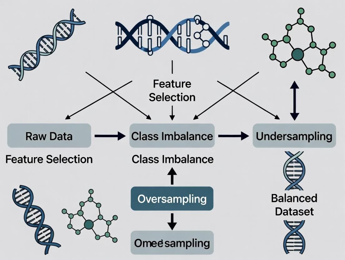
Diagram: Multi-Omics Imbalance Correction Workflow

The Scientist's Toolkit: Research Reagent Solutions

Reagent / Tool	Function in Class Imbalance Context
imbalanced-learn (Python library)	Provides implementations of SMOTE, ADASYN, Random Under/Oversampling, and ensemble methods like BalancedRandomForest. Essential for data-level interventions.
Class Weight Parameter (class_weight='balanced' in scikit-learn)	A simple, effective algorithmic approach that adjusts the loss function to penalize minority class misclassification more heavily.
PyTorch WeightedRandomSampler	A sampler for use with DataLoader that ensures a balanced batch composition during deep learning training, crucial for multi-omics models.
XGBoost / LightGBM scale_pos_weight	A parameter to set in gradient boosting frameworks to automatically adjust for imbalance by weighting the positive (minority) class.
Precision-Recall Curve (PRC) Plot	The primary visual diagnostic tool. A curve hugging the top-right indicates good performance on the minority class. More informative than ROC for imbalance.
Synthetic Data Generators (e.g., CTAB-GAN+, OMICSPred)	Advanced tools for generating realistic synthetic multi-omics data to augment minority classes, though validation is critical.

Troubleshooting Guides and FAQs

Q1: During multi-omics integration for rare disease classification, my model achieves 99% accuracy but fails to identify any true positive rare disease cases. What is wrong? A: This is a classic sign of severe class imbalance where the model defaults to predicting the majority class. Accuracy is a misleading metric here. You must switch to metrics like Precision-Recall AUC, F1-score (for the rare class), or Matthews Correlation Coefficient (MCC). Re-balance your training data using techniques like SMOTE-NC (for mixed data types) on the training set only, or use algorithmic approaches like cost-sensitive learning where misclassifying a rare disease sample incurs a higher penalty.

Q2: When subtyping cancer using RNA-seq and DNA methylation data, the clusters are driven by technical batch effects rather than biology. How can I correct this? A: Batch integration is critical. For multi-omics clustering, do not correct each dataset separately. Use integrative methods designed for this:

• Pre-processing: Apply combat or SVA on individual omics layers if batches are known.
• Integration & Clustering: Use a tool like MOFA+ (Multi-Omics Factor Analysis) to decompose variations across omics into factors. Then, cluster on the shared factor space. Alternatively, use SNF (Similarity Network Fusion) to create patient similarity networks for each omics type and fuse them.
• Validation: Ensure clusters are significant in survival analysis (log-rank test) and check known subtype markers align with clusters, not batch IDs.

Q3: My treatment response prediction model from proteomic and clinical data is overfitting despite using regularization. What steps can I take? A: Overfitting in high-dimensional, small-sample omics data is common. Implement a strict nested cross-validation (CV) protocol.

• Outer Loop: For performance estimation (e.g., 5-fold CV).
• Inner Loop: Within each training fold of the outer loop, perform another CV (e.g., 5-fold) to tune hyperparameters (like lambda for LASSO).
• Feature Selection: Perform feature selection within each inner loop to prevent data leakage. Use stability selection with LASSO to identify robust biomarkers.
• Data Augmentation: Consider synthetic data generation for the responsive class (if rare) using methods like CTGAN, but validate synthetic samples rigorously.

Q4: How do I handle missing data in multi-omics panels, especially when some samples lack entire omics layers? A: The strategy depends on the pattern.

• Missing at Random within a layer: Use imputation methods tailored to the data type (e.g., missForest for mixed omics, bpca for metabolomics).
• Missing Entire Omics Layers (e.g., some patients have no methylation data): Choose an integration method that handles this natively. MOFA+ is explicitly designed for this scenario and can learn a latent representation using all available data, treating the missing layer as missing values in the input matrix. Do not discard samples with partial data.

Experimental Protocols

Protocol 1: Robust Cancer Subtyping via Multi-Omics Integration (MOFA+ & SNF)

• Data Preparation: Obtain matched RNA-seq (counts), DNA methylation (M-values), and somatic mutation (binary) data for a cohort (N>100). Standardize features: log2(CPM+1) for RNA-seq, perform beta-to-M value conversion, filter mutations present in <1% and >95% of samples.
• Batch Correction: Apply ComBat_seq (for RNA-seq counts) and ComBat (for M-values) using known batch variables (e.g., sequencing run).
• MOFA+ Integration:
  • Create a MultiAssayExperiment R object.
  • Train MOFA+ model, specifying data groups and appropriate likelihoods (Gaussian for M-values, Poisson for counts, Bernoulli for mutations).
  • Determine optimal number of Factors using automatic relevance determination and visual inspection of variance explained.
  • Extract the factor matrix (N samples x K factors).
• Clustering: Apply consensus clustering (e.g., via ConsensusClusterPlus R package) on the MOFA+ factor matrix. Validate clusters with survival difference (Kaplan-Meier) and enrichment for established pathway signatures (GSVA).
• SNF Validation (Alternative/Complementary):
  • Construct patient similarity networks for each omics layer (Euclidean distance -> affinity matrix).
  • Fuse networks using SNF (SNFtool R package).
  • Perform spectral clustering on the fused network. Compare results to MOFA+ clusters using Adjusted Rand Index.

Protocol 2: Predicting Rare Disease Status from WGS and Clinical Data

• Cohort Definition: Case: Rare disease patients (N~50). Controls: Filtered healthy cohorts from public databases (e.g., gnomAD), matched for ancestry and sequencing platform. Note the extreme imbalance (e.g., 1:100).
• Variant Feature Engineering: From Whole Genome Sequencing (WGS), extract: (a) Rare variant burden per gene (MAF<0.001), (b) Predicted deleterious variants (CADD score >20), (c) Pathway burden scores (aggregate variants per HPO-relevant pathway).
• Data Re-balancing (Training Set Only): Split data 80/20, stratifying by case status. On the training set, apply SMOTE-NC (Synthetic Minority Over-sampling Technique for Nominal and Continuous) to synthesize rare disease cases. Do not apply to the test set.
• Model Training & Evaluation:
  • Use a tree-based model like XGBoost with scaleposweight parameter set to (number of controls / number of cases) in the original training data.
  • Train on the SMOTE-augmented training set.
  • Evaluate on the held-out, original (un-synthetically augmented) test set. Report: Precision-Recall Curve, AUC-PR, Recall (Sensitivity) at fixed high precision (e.g., 80%), and F1-score for the rare class.

Visualizations

Title: Rare Disease Prediction Workflow with Imbalance Correction

Title: Multi-Omics Cancer Subtyping Integration Pathways

Table 1: Performance Metrics for Imbalanced Learning Scenarios

Scenario	Accuracy	AUC-ROC	AUC-PR (Minority Class)	F1-Score (Minority)	Recommended Metric
Rare Disease (1:100) - Naive	0.99	0.65	0.08	0.01	AUC-PR
Rare Disease - with SMOTE	0.93	0.89	0.45	0.60	AUC-PR & F1
Cancer Subtype (Balanced)	0.85	0.92	0.86	0.84	Balanced Accuracy
Treatment Response (1:3)	0.82	0.78	0.52	0.55	AUC-PR & Recall at Precision

Table 2: Comparison of Multi-Omics Integration Tools

Tool	Methodology	Handles Missing Layers	Output for Clustering	Best For
MOFA+	Statistical Factor Analysis	Yes	Latent Factor Matrix (continuous)	Global view of variation, missing data, large K (>3 omics)
SNF	Network Fusion	No	Fused Similarity Network	Pairwise patient relations, strong complementarity
iCluster	Joint Latent Variable Model	No	Integrated Cluster Assignment	Distinct subtype discovery, penalized integration
MCIA	Multivariate Analysis	No	Component Scores	Co-inertia analysis, visualizing omics correlations

The Scientist's Toolkit: Research Reagent Solutions

Item/Category	Function in Multi-Omics Imbalance Research
Synthetic Minority Over-sampling Technique (SMOTE-NC)	Generates synthetic samples for the rare class in mixed data (continuous + categorical), mitigating imbalance in training.
Cost-Sensitive Learning Algorithms (e.g., XGBoost scale_pos_weight)	Algorithmically adjusts the penalty for misclassifying minority class samples during model training.
Stability Selection with LASSO	Robust feature selection method that identifies biomarkers consistently across resamples, reducing overfitting.
MOFA+ (Multi-Omics Factor Analysis)	Bayesian framework for integrating multiple omics datasets, capable of handling missing data and providing interpretable latent factors.
ConsensusClusterPlus R Package	Provides stable, consensus-based clustering results from high-dimensional data, essential for robust subtype definition.
Precision-Recall (PR) Curve Analysis	Evaluation framework that gives a realistic picture of model performance for imbalanced classification tasks.
Pathway Burden Scoring Scripts	Custom pipelines to aggregate rare genetic variants (e.g., from WGS) into gene sets or biological pathways for feature reduction.
ComBat/SVA (Surrogate Variable Analysis)	Batch effect correction tools critical for removing technical confounders before integration, improving biological signal.

Technical Support Center

Troubleshooting Guide & FAQs

Q1: My multi-omics classifier achieves >95% accuracy on my dataset, but fails completely on an independent validation cohort. What is the most likely cause and how can I diagnose it? A: This is a classic symptom of a model learning spurious correlations from a severely imbalanced dataset, rather than true biological signal. To diagnose:

• Generate and examine a confusion matrix on your training/held-out test set.
• Use SHAP (SHapley Additive exPlanations) or a similar feature importance method on the failed validation samples. If the top features are non-biological batch effects or rare artefacts, imbalance is the culprit.
• Check the distribution of classes between your original and validation cohorts. A significant shift indicates the model did not generalize.

• Protocol: Confusion Matrix & SHAP Analysis
  • Step 1: After model training, predict on your held-out test set. Use sklearn.metrics.confusion_matrix to visualize performance per class.
  • Step 2: Install the shap library. Create a SHAP explainer (e.g., TreeExplainer for tree-based models) using your trained model.
  • Step 3: Calculate SHAP values for a subset of your validation cohort samples (e.g., 100 samples).
  • Step 4: Use shap.summary_plot to display global feature importance. Features driving predictions for the minority class in erroneous samples are likely spurious.

Q2: What are the most effective algorithmic techniques to handle severe class imbalance (e.g., 1:100) in multi-omics integration? A: No single technique is universally best. A combination is required, prioritized as follows:

• Resampling at the Algorithm Level: Use ensemble methods designed for imbalance (e.g., Balanced Random Forest, XGBoost with scale_pos_weight parameter tuned).
• Cost-sensitive Learning: Explicitly assign higher misclassification costs to the minority class during model training.
• Resampling at the Data Level: Use SMOTE-ENN (Synthetic Minority Over-sampling Technique followed by Edited Nearest Neighbors) rather than simple oversampling, as it generates synthetic samples and cleans noisy data. Avoid simple random undersampling of the majority class in omics, as it discards potentially critical biological information.

• Protocol: Implementing SMOTE-ENN with Balanced Random Forest

Q3: How do I choose the right performance metric when evaluating models on imbalanced omics data? A: Accuracy is misleading. Use metrics that are robust to class distribution. The table below summarizes key metrics:

Metric	Formula (Simplified)	When to Use	Pitfall in Imbalance
Balanced Accuracy	(Sensitivity + Specificity) / 2	General replacement for accuracy.	Can be overly optimistic if one class is extremely rare.
Matthews Correlation Coefficient (MCC)	(TP×TN - FP×FN) / √((TP+FP)(TP+FN)(TN+FP)(TN+FN))	Best overall metric for binary classification, robust to imbalance.	Less intuitive than precision/recall.
Precision-Recall AUC	Area under the Precision-Recall curve.	Primary metric for severe imbalance. Focuses on minority class performance.	Does not evaluate true negative performance.
F-Beta Score	(1+β²) * (PrecisionRecall) / (β²Precision + Recall)	When you want to weight precision (β<1) or recall (β>1) higher.	Requires choosing an appropriate β value.

Q4: I suspect my "biomarker" is an artefact of batch effect confounded with class imbalance. How can I test this? A: Conduct a permutation-based batch effect correction analysis.

• Protocol: Batch Effect Permutation Test
  • Record the original p-value/importance score of your putative biomarker.
  • Shuffle the batch labels of your samples while keeping the class labels intact. This breaks any true association between batch and class.
  • Re-run your entire feature selection and model training pipeline on this permuted data.
  • Repeat steps 2-3 at least 100 times.
  • Compare your original biomarker's score to the distribution of scores from the permuted datasets. If the original score falls within the 95% percentile of the null distribution, it is likely a batch artefact.

The Scientist's Toolkit: Research Reagent Solutions

Item / Solution	Function in Imbalanced Multi-Omics Research
Imbalanced-Learn (Python library)	Provides a suite of resampling algorithms (SMOTE, SMOTE-ENN, Tomek Links) for preprocessing. Essential for data-level correction.
SHAP / LIME Libraries	Model-agnostic explainability tools to audit which features drive predictions for minority class samples, identifying spurious correlations.
ComBat or ComBat-seq (R)	Batch effect correction tools that preserve biological signal. Critical for removing technical variance that can be magnified by imbalance.
scikit-learn with class_weight='balanced'	Enables built-in cost-sensitive learning for many algorithms, penalizing model errors on the minority class more heavily.
MLxtend or Custom Pipelines	For implementing nested cross-validation correctly within resampling loops, preventing data leakage and over-optimistic performance estimates.

Experimental & Conceptual Visualizations

Diagram 1: Spurious Correlation in Imbalanced Data

Diagram 2: Robust Workflow for Imbalanced Multi-Omics

Technical Support Center: Troubleshooting Multi-Omics Integration & Class Imbalance

FAQs & Troubleshooting Guides

Q1: During integration of my genomic (SNP), transcriptomic (RNA-Seq), and proteomic (LC-MS/MS) data for a disease vs. control study, my classifier consistently predicts the majority class (control). What are the primary technical checkpoints? A: This is a classic symptom of class imbalance compounded by multi-omic batch effects. Follow this checklist:

• Per-omics Balance Check: Ensure imbalance isn't severe within each data layer before integration. For RNA-Seq, use DESeq2's median-of-ratios normalization, which handles imbalance better than TPM/RPKM alone.
• Batch Effect Diagnosis: Perform PCA on each omic layer separately, colored by batch_id and class_label. Strong clustering by batch_id often swamps the class signal.
• Integration Method Audit: If using early integration (concatenating features), the high-dimensional majority class noise dominates. Shift to intermediate (e.g., MOFA+) or late integration (ensemble classifiers per omic) approaches.

Q2: What are the best practices for synthetic data generation (e.g., SMOTE) in a multi-omics context? Can I apply it to the concatenated feature matrix? A: Do not apply SMOTE directly to a concatenated multi-omics matrix. This ignores the distinct statistical distributions of each omics layer and creates unrealistic synthetic samples. The preferred protocol is:

• Strategy: Apply synthetic oversampling separately within each omics data layer for the minority class samples, prior to integration.
• Protocol: For transcriptomics count data, use methods like ROSE or SMOTE-NC that handle categorical/continuous mixes. For proteomics (continuous, often normal-ish), standard SMOTE is acceptable.
• Critical Step: Maintain strict sample alignment. A synthetic sample S1_rna generated from biological sample B1 must be linked to the same sample's proteomic data (B1_prot). Do not generate new synthetic proteomics for S1_rna.

Q3: Our differential expression (transcriptomics) and differential abundance (proteomics) lists show poor concordance for the minority class (rare disease). Is this a technical artifact or likely biology? A: First, rule out technical causes using this workflow:

• Normalization Review:
  • Transcriptomics: Use a normalization method robust to extreme imbalance, such as trimmed mean of M-values (TMM) in edgeR or DESeq2's median ratio method.
  • Proteomics: For label-free LC-MS/MS, ensure normalization like quantile or cyclic loess is applied. Verify normalization separately within each condition before comparing across conditions.
• Imputation Audit: In proteomics, missing values are not random (MNAR) for low-abundance proteins in the minority class. Standard k-NN imputation creates false positives. Use methods like Adaptive Bayesian (AB) imputation or DirectMNAR designed for MNAR data.
• Statistical Power Check: The minority class likely has insufficient power for proteomics. See Table 1.

Table 1: Key Quantitative Challenges in Imbalanced Multi-Omics Studies

Challenge	Typical Impact on Minority Class	Data-Driven Threshold for Concern
Proteomic Coverage	>30% missing data (MNAR) in minority class samples.	Missingness rate > 1.5x that of majority class.
Statistical Power (Proteomics)	< 5 samples in minority class rarely detects <2-fold change.	Need ≥ 8 minority samples for 80% power at FDR=0.05.
Feature Concordance	< 20% overlap in DE genes & DA proteins.	Expect ~40% overlap in balanced studies.
Batch Effect Strength	PCA shows batch explaining >50% of variance vs. class <10%.	Batch variance > 2x class variance is critical.

Experimental Protocol: Validating Multi-Omics Integration Amidst Imbalance Title: Protocol for Multi-Omics Data Fusion with Class Imbalance Evaluation. Objective: To integrate disparate omics layers while diagnosing and mitigating bias from class imbalance. Steps:

• Pre-processing & Individual Layer Analysis:
  • Genomics (SNPs): Perform QC, imputation, and encode as additive allele dosages. Check minor allele frequency (MAF) – rare variants in the minority class will be discarded by standard MAF>0.01 filters.
  • Transcriptomics (RNA-Seq): Trim, align, and generate counts. Use DESeq2 with a balanced design matrix (~ batch + class) for preliminary DE analysis. Note the dispersion estimates for minority class.
  • Proteomics (LFQ): Process with MaxQuant or DIA-NN. Apply sample-specific normalization and use limma or DEqMS with weighted options for DA testing.
• Imbalance-Specific Normalization: Apply ComBat or Harmony separately to each omics layer, using class as the primary covariate and batch as the adjustment variable to prevent signal removal.
• Intermediate Integration with MOFA+: Run MOFA2 creating a single model with all three data types. Critically inspect the variance explained by Factor 1 per view. If the majority class dominates a factor, use the groups parameter to train a model per condition and integrate factors.
• Downstream Analysis & Validation:
  • Use the MOFA+ factors (latent variables) as input features for a classifier (e.g., SVM).
  • Apply stratified nested cross-validation, where the inner loop includes resampling (SMOTE) only on the training fold.
  • Performance Metrics: Report Balanced Accuracy, Matthews Correlation Coefficient (MCC), and AUPRC alongside standard AUC. AUPRC is crucial for imbalanced scenarios.

Visualizations

Diagram 1: Multi-Omics Integration Pathways & Imbalance Pitfalls

Diagram 2: SMOTE Protocol for Multi-Omics Data

The Scientist's Toolkit: Research Reagent Solutions

Reagent / Tool	Function in Imbalanced Multi-Omics	Key Consideration
DESeq2 (R)	Differential expression analysis for RNA-Seq.	Its median-of-ratios normalization and dispersion estimation are more stable under moderate imbalance than TPM + t-test.
MOFA+ (R/Python)	Multi-Omics Factor Analysis for unsupervised integration.	Use the groups argument to model classes separately, preventing majority class domination of factors.
Harmony (R)	Batch effect correction.	Corrects per-omics layer while preserving biological signal (like minority class), better than ComBat for severe imbalance.
scikit-learn imblearn	Synthetic oversampling (SMOTE variants).	Use SMOTE-NC for mixed data (transcriptomics with clinical covariates). Never apply post-integration.
MissForest (R)/ DIA-NN (SW)	Handles MNAR missing data in proteomics.	Critical for minority class where low-abundance proteins are systematically missing. Avoid k-NN imputation.
Limma with voom (R)	DE analysis for proteomics or RNA-Seq.	Use limma with voom for RNA-Seq or lmFit for proteomics; allows weighting to address heterogeneity in minority class.

Troubleshooting Guides & FAQs

Q1: In my imbalanced multi-omics classification (e.g., rare disease vs. control), my model achieves 98% accuracy, but I am missing all the rare disease cases. What is happening and which metric should I prioritize? A: This is a classic symptom of the "accuracy paradox" in imbalanced datasets. A model can achieve high accuracy by simply predicting the majority class (controls) for all samples. Accuracy is misleading here. You must prioritize Recall (Sensitivity) for the minority class. Recall measures the proportion of actual positive cases (rare disease) correctly identified. A high accuracy with zero minority class recall indicates a useless model for your primary goal of finding rare disease signals.

Q2: When I optimize for high recall on my minority cancer subtype from integrated RNA-seq and methylation data, my model starts predicting many false positives (healthy tissues as cancerous). How can I balance this? A: Increasing recall often decreases Precision (the proportion of positive predictions that are correct). You are now capturing more true cancers but also mislabeling healthy samples. To balance precision and recall, optimize for the F1-Score, which is their harmonic mean. Use the F1-score for the minority class as your key metric to select models. Alternatively, use the Precision-Recall (PR) curve and its summary metric, Area Under the PR Curve (AUC-PR), which remains informative under severe imbalance, unlike the ROC-AUC.

Q3: How do I interpret an AUC-PR score of 0.25 versus an AUC-ROC score of 0.85 for the same model on my proteomics data? A: In imbalanced scenarios, AUC-ROC can be overly optimistic because the high number of true negatives (majority class) inflates the False Positive Rate axis. An AUC-ROC of 0.85 may still represent poor performance on the minority class. The AUC-PR focuses solely on the performance concerning the positive (minority) class, making it more critical. An AUC-PR of 0.25 is generally poor and indicates significant difficulty in reliably identifying positive cases. Prioritize improving your model's AUC-PR.

Q4: What is a concrete experimental protocol to evaluate metrics properly in a class-imbalanced multi-omics experiment? A: Follow this stratified protocol:

• Data Split: Perform a stratified split (e.g., 70/15/15) to maintain class imbalance ratios in training, validation, and test sets.
• Model Training: Train your classifier (e.g., Random Forest, XGBoost, neural network) on the training set. Consider using class weighting, oversampling (SMOTE), or ensemble methods designed for imbalance.
• Validation & Threshold Tuning: On the validation set, generate predicted probabilities. Do not use the default 0.5 threshold. Generate a Precision-Recall curve. Based on your research cost/benefit (e.g., cost of a false positive vs. missing a true positive), select an optimal probability threshold.
• Final Evaluation: Apply the chosen threshold to the held-out test set. Calculate the confusion matrix and derive class-specific Precision, Recall, and F1-scores. Report the AUC-PR (which is threshold-agnostic).

Q5: My collaborator insists on using ROC curves. How do I explain why PR curves are better for our single-cell multi-omics integration study with rare cell types? A: Explain that the ROC curve plots True Positive Rate (Recall) vs. False Positive Rate. FPR becomes dominated by the vast number of majority class cells, making the curve look artificially good. The PR curve plots Precision vs. Recall, both of which are focused on the performance regarding the rare cell type of interest. Shifts in class distribution (like changing the number of background cells) do not affect the PR curve's interpretability for the target class, making it the standard for imbalanced detection tasks.

Metric	Formula	Focus	Best Used When...	Pitfall in Imbalance
Accuracy	(TP+TN)/(TP+TN+FP+FN)	Overall correctness	Classes are perfectly balanced.	Highly misleading; inflated by majority class.
Precision	TP/(TP+FP)	Reliability of a positive prediction.	Cost of False Positive is high (e.g., costly follow-up assay).	Can be high even if many positives are missed (low recall).
Recall (Sensitivity)	TP/(TP+FN)	Coverage of actual positive cases.	Cost of False Negative is high (e.g., missing a disease biomarker).	Can be high at the expense of many false alarms (low precision).
F1-Score	2 * (Precision*Recall)/(Precision+Recall)	Balance between Precision & Recall.	Seeking a single metric to compare models for the minority class.	Assumes equal weight of Precision and Recall; may not align with clinical utility.
AUC-ROC	Area under ROC curve	Overall ranking performance across all thresholds.	Comparing models where both classes are of equal interest.	Overly optimistic with large class imbalance.
AUC-PR	Area under Precision-Recall curve	Performance focused on the positive (minority) class.	The standard for imbalanced datasets in multi-omics.	No inherent baseline; random performance is the % of positives.

Experimental Protocol: Evaluating Classifiers for Imbalanced Multi-Omics Data

Objective: To rigorously train and evaluate a machine learning model for rare subtype prediction from integrated omics data, using metrics robust to class imbalance.

Materials: Integrated multi-omics dataset (e.g., RNA-seq, methylation, proteomics), computational environment (Python/R), libraries (scikit-learn, imbalanced-learn, XGBoost).

Methodology:

• Preprocessing & Integration: Perform omics-specific normalization, batch correction, and feature selection. Use methods like MOFA or concatenation for integration.
• Stratified Data Partitioning: Split the integrated feature matrix and corresponding labels into Training (70%), Validation (15%), and Test (15%) sets using StratifiedShuffleSplit to preserve the minority class ratio.
• Model Training with Imbalance Adjustment: Train a classifier (e.g., XGBClassifier) on the training set. Mandatory: Set scale_pos_weight parameter or use class_weight='balanced' in scikit-learn. Alternatively, apply SMOTE from the imblearn library only on the training fold.
• Validation & Threshold Optimization:
  • Use the trained model to predict probabilities for the positive class (minority) on the Validation set.
  • Calculate precision and recall values across all probability thresholds.
  • Plot the Precision-Recall curve. Calculate the AUC-PR.
  • Based on the PR curve and project goals, select an optimal threshold (e.g., threshold that yields a recall of at least 0.8 for the highest possible precision).
• Final Test Set Evaluation:
  • Apply the optimal threshold from step 4 to the probabilities predicted for the held-out Test set.
  • Generate the final confusion matrix.
  • Calculate and report: Minority Class Precision, Recall, and F1-score. Report the AUC-PR (calculated directly from the probabilities, not the thresholded predictions).
• Comparison & Reporting: Compare multiple models (e.g., Random Forest, SVM, Neural Net) based primarily on their Test Set AUC-PR and Minority Class F1-score.

Visualizations

Title: Experimental Workflow for Imbalanced Multi-Omics Analysis

Title: Decision Guide for Choosing Metrics in Imbalanced Data

The Scientist's Toolkit: Research Reagent & Computational Solutions

Item / Solution	Function in Imbalanced Multi-Omics Research
imbalanced-learn (Python library)	Provides algorithms like SMOTE, ADASYN, and SMOTE-ENN for synthetic minority oversampling and data cleaning directly in computational pipelines.
scale_pos_weight (XGBoost parameter)	A key parameter to scale the gradient for the positive class, effectively penalizing misclassifications of the minority class more heavily during model training.
Stratified K-Fold Cross-Validation	A data splitting method that ensures each fold retains the same percentage of minority class samples as the full dataset, preventing skewed evaluation.
Precision-Recall Curve (Plot)	A diagnostic visualization tool to understand the trade-off between precision and recall at different classification thresholds for the minority class.
Cost-Sensitive Learning Algorithms	Modified versions of standard classifiers (e.g., Random Forest, SVM) that assign a higher penalty to errors made on the minority class during the learning process.
Ensemble Methods (e.g., RUSBoost)	Combines random under-sampling of the majority class with a boosting algorithm to improve model focus on difficult-to-classify minority samples.
MOFA+ (Multi-Omics Factor Analysis)	A Bayesian framework for multi-omics integration that can handle missing data and provides a lower-dimensional latent representation, useful as input for classifiers.

Balancing the Scales: A Toolkit of Data-Level, Algorithm-Level, and Hybrid Techniques

Technical Support Center

Troubleshooting Guides

Issue 1: SMOTE Generates Noisy Synthetic Samples in High-Dimensional Multi-Omics Data

• Symptoms: Model performance (e.g., AUC-ROC) decreases after applying SMOTE. Synthetic samples appear as outliers in PCA plots.
• Diagnosis: The "curse of dimensionality" leads to inaccurate distance metrics in the feature space, causing SMOTE to generate samples in sparse, irrelevant regions.
• Solution: Apply feature selection (e.g., variance filter, LASSO) or dimensionality reduction (e.g., PCA, UMAP) before SMOTE. Use SMOTEENN (SMOTE + Edited Nearest Neighbors) to clean the data post-synthesis.

Issue 2: ADASYN Causes Overfitting to Specific Minority Subclusters

• Symptoms: Excellent training accuracy but poor validation/hold-out test set performance. Over-representation of certain minority samples is observed.
• Diagnosis: ADASYN's density-based weighting excessively focuses on hard-to-learn subclusters, creating an unrealistic local distribution.
• Solution: Tune the n_neighbors parameter in ADASYN to a higher value. Combine ADASYN with standard undersampling of the majority class (e.g., RandomUnderSampler) to balance the emphasis.

Issue 3: Tomek Links Over-Reduce Dataset Leading to Loss of Critical Majority Class Information

• Symptoms: Drastic reduction in dataset size, potentially removing informative majority class samples crucial for robust model generalization.
• Diagnosis: In complex, overlapping multi-omics class distributions, many majority samples form Tomek links with minority samples.
• Solution: Do not use Tomek Links alone. Use it as a cleaning step after oversampling (SMOTE/ADASYN) via SMOTETomek. Set sampling_strategy for Tomek Links to only remove majority class samples from the link pair.

Issue 4: Memory/Computational Error During SMOTE on Large Multi-Omics Matrices

• Symptoms: Kernel crashes or "MemoryError" when fitting SMOTE on large datasets (e.g., >20,000 features x 10,000 samples).
• Diagnosis: The k-NN algorithm becomes computationally prohibitive in high-dimensional space.
• Solution: Use the random_state for reproducibility and batch processing. Employ the SVMSMOTE or BorderlineSMOTE variants, which can be more efficient by focusing on boundary samples. Consider using a dedicated library like imbalanced-learn (scikit-learn-contrib).

Frequently Asked Questions (FAQs)

Q1: Should I apply SMOTE/ADASYN to my entire multi-omics dataset before splitting it into train and test sets? A: Absolutely not. This causes data leakage, as synthetic samples based on test set information can inflate performance. Always apply resampling techniques only within the training fold during cross-validation or after a initial train-test split. The test set must remain completely unseen and unmodified.

Q2: Which strategy is best for my integrated transcriptomics and metabolomics data: SMOTE or ADASYN? A: There is no universal best. ADASYN may be preferable if the minority class is highly heterogeneous, as it focuses on harder-to-learn sub-types. SMOTE is simpler and more reproducible. The recommended protocol is to create a pipeline and validate performance using nested cross-validation, comparing both against a baseline with no resampling. See the comparative table below.

Q3: How do I choose parameters like k_neighbors for SMOTE in a multi-omics context? A: Start with a low k_neighbors (e.g., 5) to avoid synthesizing from distant, potentially irrelevant neighbors in high-D space. Treat k_neighbors as a hyperparameter and optimize it within your cross-validation loop. Use odd numbers to avoid ties.

Q4: Can Tomek Links be used to completely solve class imbalance? A: No. Tomek Links is primarily a data cleaning technique, not a resampling technique for severe imbalance. Its purpose is to remove ambiguous, overlapping samples from the majority class to better define class boundaries. It is most effective when combined with oversampling methods.

Q5: How do I evaluate if SMOTE/ADASYN improved my model beyond accuracy? A: Accuracy is misleading with imbalance. Always use metrics that are robust to imbalance:

• Precision-Recall Curve (PRC) and Area Under PRC (AUPRC): Primary metric for imbalanced data.
• ROC-AUC: Useful but can be optimistic.
• Balanced Accuracy: (Sensitivity + Specificity) / 2.
• F1-Score / Geometric Mean (G-Mean): Harmonized metrics. Compare these metrics on your held-out test set before and after applying the strategy.

Comparative Analysis of Resampling Strategies

Table 1: Quantitative Comparison of SMOTE, ADASYN, and Tomek Links

Feature	SMOTE	ADASYN	Tomek Links
Primary Goal	Synthetic Oversampling	Synthetic Oversampling	Data Cleaning (Undersampling)
Key Mechanism	Interpolates between minority samples.	Weighted interpolation focusing on "hard" samples.	Removes majority class samples in Tomek pairs.
Impact on Dataset Size	Increases (adds synthetic samples).	Increases (adds synthetic samples).	Decreases (removes real samples).
Risk of Overfitting	Moderate	Higher (can overfit to noise)	Low
Parameter Sensitivity	k_neighbors	k_neighbors, density estimation	Distance metric
Best Suited For	Relatively homogeneous minority classes.	Heterogeneous minority classes with subclusters.	Cleaning boundaries post-oversampling.

Experimental Protocols

Protocol 1: Benchmarking Resamplers with Nested Cross-Validation

Objective: To rigorously evaluate the impact of SMOTE, ADASYN, and Tomek Links on classifier performance for a multi-omics dataset.

• Data Preprocessing: Perform initial quality control, normalization, and batch correction specific to each omics layer (e.g., RNA-seq, proteomics). Integrate layers via concatenation or multi-view methods.
• Initial Split: Hold out 20% of the data as a final, untouched test set.
• Nested CV Loop:
  • Outer Loop (Performance Estimation): 5-fold CV on the 80% training data.
  • Inner Loop (Model Selection): On each outer training fold, perform 3-fold CV to: a. Apply a resampling strategy (e.g., SMOTE) only to the inner training fold. b. Train a classifier (e.g., Random Forest, XGBoost). c. Tune hyperparameters (including resampler parameters like k_neighbors).
  • Evaluation: Train the best inner model on the entire outer training fold (with resampling) and evaluate on the outer test fold. Use AUPRC as the scoring metric.
• Final Evaluation: Train the best overall pipeline on the entire 80% training set and evaluate on the held-out 20% test set. Report AUPRC, Balanced Accuracy, and F1-Score.

Protocol 2: Implementing SMOTETomek for Integrated Genomics and Metabolomics Data

Objective: To balance a dataset and clean class boundaries for a disease vs. control classification task.

• Input: Integrated feature matrix (e.g., X = gene expression + metabolite abundances, y = disease labels (imbalanced)).
• Pipeline Definition (Python using imbalanced-learn):

• Execution: Fit the pipeline on the training data. The SMOTETomek object will first apply SMOTE to the minority class, then remove Tomek links from both classes (primarily majority).

Visualizations

Diagram 1: SMOTE Algorithm Workflow for a Single Minority Sample

Diagram 2: Decision Boundary Cleaning with Tomek Links

Diagram 3: Integrated Multi-Omics Resampling Pipeline

The Scientist's Toolkit: Research Reagent Solutions

Table 2: Essential Computational Tools for Imbalance Correction in Multi-Omics

Tool / Package	Function	Key Use-Case in Multi-Omics
imbalanced-learn (Python)	A comprehensive library offering SMOTE, ADASYN, Tomek Links, and combined methods.	Primary library for implementing all data-level resampling strategies in a scikit-learn compatible pipeline.
scikit-learn	Core machine learning library providing classifiers, metrics, and preprocessing modules.	Used for model training, hyperparameter tuning (GridSearchCV), and evaluation metrics (precisionrecallcurve).
MultiOmicsIntegration Tool (e.g., MOFA2)	Statistical framework for integrating multi-omics data into a lower-dimensional representation.	Generating integrated latent factors that can be resampled, mitigating the high-dimensionality challenge for SMOTE.
Conda / Pip	Package and environment management systems.	Ensuring reproducible environments with specific versions of imbalanced-learn, scikit-learn, and omics analysis packages.
Jupyter Notebook / RMarkdown	Interactive computational notebooks for literate programming.	Documenting the complete analytical workflow, from data loading and resampling to model evaluation, ensuring full reproducibility.

Troubleshooting Guides & FAQs

Q1: My cost-sensitive classifier is still biased towards the majority class, despite assigning higher misclassification costs to the minority class. What could be wrong?

A: This common issue often stems from improper cost matrix calibration. The assigned costs may be dominated by the class distribution itself. Verify your cost matrix by ensuring the expected cost of predicting any class is normalized. A recommended diagnostic is to compute the cost-adjusted prior distribution: ( P{adj}(y) \propto P(y) \times C(y, \hat{y}) ), where ( C ) is the cost of misclassifying true class ( y ). If ( P{adj} ) is still skewed, iteratively adjust costs. Additionally, ensure your learning algorithm truly minimizes the cost-sensitive loss (e.g., use class_weight='balanced_subsample' in sklearn ensemble methods for large datasets).

Q2: How do I set appropriate Bayesian priors for multi-omics features when prior biological knowledge is sparse or conflicting?

A: For sparse knowledge, use weakly informative or regularization priors. For genomic count data (e.g., RNA-Seq), a log-normal or Gamma prior can stabilize variance. For conflicting knowledge, a hierarchical prior structure is effective. For example, define a prior where the mean ( \muk ) for a feature's effect in omics type ( k ) is drawn from a global distribution: ( \muk \sim N(\mu_{global}, \tau^2) ). This allows sharing of statistical strength across omics layers. Set hyperpriors on ( \tau ) to control the degree of borrowing.

Q3: When integrating cost-sensitive learning with Bayesian models, how do I prevent the model likelihood from being overwhelmed by the cost weights?

A: Integrate costs at the decision rule level, not the likelihood level. Build your model with standard Bayesian priors and obtain the posterior predictive distribution ( P(y^* | X^, D) ). Then, during prediction, apply the cost matrix to this distribution to make the decision that minimizes the expected risk: ( \hat{y} = \arg\min_{\hat{y}} \sum_{y} P(y^=y | X^*, D) \cdot C(y, \hat{y}) ). This separates inference from decision theory cleanly.

Q4: I'm getting poor performance with cost-sensitive deep learning on imbalanced omics data. What architectural or training adjustments should I consider?

A: First, apply class-weighted loss functions (e.g., Weighted Cross-Entropy) where the weight for class ( i ) is often set to ( wi = \text{totalsamples} / (\text{numclasses} * \text{samplesinclass}i) ). Second, combine this with Bayesian layers (e.g., Monte Carlo Dropout) to obtain uncertainty estimates and perform cost-sensitive decision-making post-inference as in Q3. Third, ensure batch sampling is balanced (e.g., use a BalancedBatchGenerator) to prevent gradient bias.

Experimental Protocols

Protocol 1: Calibrating a Cost Matrix for Imbalanced Multi-Omics Classification

Objective: Systematically determine a cost matrix for a Support Vector Machine (SVM) to classify rare disease subtypes from integrated genomics and proteomics data.

• Data Partition: Split integrated omics dataset (e.g., 500 samples, 5% minority class) into 60% training, 20% validation, 20% test. Stratify splits.
• Baseline: Train a standard SVM with RBF kernel. Evaluate on validation set using F2-Score (emphasizing recall).
• Initial Cost Grid: Define a cost ratio ( R = C{minority}/C{majority} ). Test ( R ) values = [5, 10, 25, 50, 100] where ( C_{majority} = 1 ). For each ( R ), train a cost-sensitive SVM.
• Validation & Adjustment: Select the ( R ) yielding the highest validation F2-Score. If precision collapses (>50% drop from baseline), add a constraint: reduce ( R ) until precision drop is ≤30%.
• Final Evaluation: Retrain on combined training+validation set with the selected cost matrix. Report final metrics on the held-out test set.

Protocol 2: Incorporating Hierarchical Bayesian Priors for Feature Selection

Objective: Integrate pathway knowledge as priors to select discriminative features across transcriptomics and metabolomics data.

• Prior Definition: For each feature ( j ), encode its known pathway membership. Use a spike-and-slab prior: ( \betaj \sim (1-\pij) \delta0 + \pij N(0, \sigma^2) ). Set the inclusion probability ( \pi_j ) higher (e.g., 0.8) for features in disease-associated pathways (from KEGG, Reactome).
• Model Specification: Use a Bayesian logistic regression model. For metabolomics features with less reliable annotation, place a hyperprior on their ( \pij ): ( \pij \sim \text{Beta}(2, 5) ).
• Inference: Perform Markov Chain Monte Carlo (MCMC) sampling (e.g., using PyMC3 or Stan) to obtain posterior distributions of ( \beta_j ).
• Selection: A feature is deemed selected if its posterior probability ( P(\beta_j \neq 0 | Data) > 0.95 ). Compare the list against a baseline model with non-informative priors.

Table 1: Comparison of Algorithm-Level Approaches on Imbalanced Multi-Omics Datasets

Dataset (Minority %)	Method	Balanced Accuracy	F1-Score (Minority)	Expected Cost (↓)	AUC-ROC
TCGA-BRCA Subtype (8%)	Standard SVM	0.62	0.21	1.00 (Baseline)	0.78
	Cost-SVM (R=25)	0.75	0.45	0.48	0.82
	Bayesian Logistic (Weak Prior)	0.70	0.38	0.67	0.85
	Cost-Sensitive Bayesian	0.78	0.52	0.41	0.87
Metabo+Proteo Cohort (12%)	Standard Random Forest	0.71	0.32	1.00 (Baseline)	0.80
	Cost-Weighted RF	0.80	0.49	0.55	0.83
	Hierarchical Bayesian Model	0.77	0.41	0.70	0.88
	Cost-Decision on Bayesian	0.82	0.55	0.50	0.90

Table 2: Typical Cost Matrix for Rare Oncogenic Pathway Detection

Actual \ Predicted	Pathway Active (Positive)	Pathway Inactive (Negative)
Pathway Active	0 (Correct)	10 (High Cost: Missed Detection)
Pathway Inactive	1 (Low Cost: False Alarm)	0 (Correct)

Visualizations

Title: Algorithm Selection Workflow for Imbalanced Data

Title: Hierarchical Bayesian Prior Structure for Multi-Omics

The Scientist's Toolkit: Research Reagent Solutions

Item / Resource	Function / Purpose in Context
imbalanced-learn (Python library)	Provides implementations of cost-sensitive learning algorithms (e.g., BalancedRandomForest, BalancedBaggingClassifier) and sampling methods.
PyMC3 / Stan (Probabilistic Programming)	Enables the specification of custom Bayesian hierarchical models with informative priors for multi-omics integration and inference.
Cost-Sensitive Evaluation Metrics (Code)	Custom scripts to calculate expected misclassification cost, weighted AUC (AUC-W), and cost curves for model selection beyond standard metrics.
Pre-defined Biological Prior Databases	KEGG, Reactome, MSigDB. Used to map omics features to pathways and biological processes for setting informed prior probabilities.
MCMC Diagnostic Tools (ArviZ, bayesplot)	Essential for assessing convergence (R-hat, effective sample size) of Bayesian models to ensure reliable posterior estimates.
Automated Hyperparameter Optimization (Optuna, Hyperopt)	Systems to efficiently search over cost ratios (R) and prior distribution hyperparameters (e.g., scale of Gaussian priors).

Technical Support Center: Troubleshooting & FAQs

Frequently Asked Questions

Q1: My Balanced Random Forest (BRF) model is still biased towards the majority class in my RNA-Seq dataset, despite undersampling. What could be wrong? A: This is often due to within-class imbalance or noisy features. In multi-omics, a majority class may have subclusters that are poorly represented. Ensure your undersampling is stratified not just by class label, but also by key biological covariates (e.g., batch, patient cohort). Pre-filter features using variance stabilization or ANOVA F-value to reduce noise before training.

Q2: When using EasyEnsemble on proteomics data, each AdaBoost ensemble seems to overfit its specific subset. How can I improve generalization? A: This indicates high variance. First, reduce the complexity of the base learners in each AdaBoost ensemble (e.g., set max_depth of decision trees to 3-5). Second, increase the number of subsets (n_estimators) to improve the law of averages. Third, apply feature selection independently for each subset to create diverse models, which often improves final ensemble performance.

Q3: How do I handle missing values in multi-omics data before applying these ensemble methods? A: Neither BRF nor EasyEnsemble natively handle missing data. You must impute. For genomics/metabolomics data:

• Use K-Nearest Neighbors (KNN) imputation within each class separately to avoid leakage.
• For missing-not-at-random data (common in metabolomics), flag features with >20% missingness and consider removing them.
• Post-imputation, apply quantile normalization to correct for any introduced distribution shifts.

Q4: My computational runtime for EasyEnsemble is extremely high on my large methylomics dataset. Any optimization strategies? A: Yes. Employ parallelization and dimensionality reduction.

• Set n_jobs=-1 to use all CPU cores.
• Perform a two-stage feature reduction: First, use a variance threshold. Second, apply a linear method like truncated SVD on each balanced subset individually, which is faster than on the full dataset.
• Consider using the random_state parameter for reproducible subsampling to avoid redundant experimentation.

Q5: How do I choose between Balanced Random Forest and EasyEnsemble for my specific multi-omics integration project? A: The choice hinges on your data size and goal.

Criterion	Balanced Random Forest (BRF)	EasyEnsemble
Primary Mechanism	Under-sampling + Bagging	Under-sampling + Bagging of Boosting Ensembles
Best For	Moderately imbalanced data (e.g., 1:10 ratio)	Severely imbalanced data (e.g., 1:100 ratio)
Computational Cost	Lower	Higher (trains multiple AdaBoost models)
Model Diversity	Moderate (via bagging)	High (via independent subsets & boosting)
Key Hyperparameter	max_samples (size of bootstrap sample)	n_estimators (number of subsets), learning_rate (of AdaBoost)
Recommended for	Initial screening, quicker prototype	Final model, maximizing AUC-PR, drug target discovery

Experimental Protocols

Protocol 1: Implementing a Balanced Random Forest for miRNA Biomarker Discovery Objective: Identify a robust miRNA signature from a class-imbalanced cohort (e.g., 30 Responders vs. 300 Non-Responders to a therapy).

• Data Preparation: Quantile normalize miRNA count data. Remove miRNAs expressed in <10% of samples.
• Feature Pre-selection: Perform a Wilcoxon rank-sum test on the training set only. Retain the top 200 miRNAs with smallest p-values.
• Model Training: Instantiate a BalancedRandomForestClassifier (from imbalanced-learn) with n_estimators=500, max_samples=0.8, max_features='sqrt', random_state=42. Use 5-fold stratified cross-validation.
• Feature Importance: Extract Gini importance from the trained model. Calculate stability of importance ranks across CV folds.
• Validation: Apply the selected miRNA signature and trained model to a held-out validation cohort. Report AUC-ROC and AUC-PR.

Protocol 2: EasyEnsemble for Integrating Transcriptomics and Methylomics in Subtype Classification Objective: Classify a rare cancer subtype (5% prevalence) using integrated omics.

• Data Integration: Perform standard normalization per platform. Use DIABLO (mixOmics R package) or MOFA to derive 10-15 latent factors from each omics layer as the integrated feature set.
• Ensemble Training: Instantiate an EasyEnsembleClassifier (from imbalanced-learn) with n_estimators=50. Set the base estimator to AdaBoostClassifier with n_estimators=30 and learning_rate=0.8.
• Balancing: Each EasyEnsemble subset will create a balanced sample (e.g., 100% of rare class, random 5% of majority class from the training fold).
• Aggregation: Use the average of probabilities from all 50 AdaBoost ensembles for final prediction.
• Evaluation: Plot the Precision-Recall curve. Calculate the F1-score and Balanced Accuracy. Perform a permutation test (1000 iterations) to assess significance of the AUC-PR.

Visualizations

BRF vs. EasyEnsemble Experimental Workflow

Logic: Choosing Between BRF and EasyEnsemble

The Scientist's Toolkit: Research Reagent Solutions

Item / Tool	Function in Imbalanced Multi-Omics Research
imbalanced-learn (Python library)	Core library providing implemented BalancedRandomForestClassifier and EasyEnsembleClassifier algorithms.
scikit-learn	Provides base estimators (DecisionTreeClassifier, AdaBoost), metrics (averageprecisionscore), and preprocessing tools.
MOFA2 (R/Python)	A tool for multi-omics factor analysis to integrate heterogeneous data types and reduce dimensionality before classification.
smote-variants (Python library)	Provides advanced oversampling techniques (e.g., SMOTE-NC) for mixed data types (continuous & categorical).
SHAP (Shapley Additive exPlanations)	Explains the output of any ensemble model, critical for interpreting feature importance in complex, imbalanced models.
MLxtend	Provides useful utilities for evaluating classifier stability and feature selection consistency across CV folds.
Custom Stratified Sampler	A script to ensure train/test splits preserve the proportion of rare classes and key clinical covariates (e.g., age, batch).

This technical support center is designed to assist researchers implementing deep learning for multi-omics data analysis, a core methodology within our broader thesis on Dealing with Class Imbalance in Multi-Omics Research. Class imbalance, where one class (e.g., healthy samples) vastly outnumbers another (e.g., rare disease subtype), is a pervasive challenge that biases models toward the majority class. This guide details the application of weighted loss functions and Focal Loss to mitigate this issue, ensuring robust biomarker discovery and patient stratification.

Troubleshooting Guides & FAQs

Q1: My neural network achieves >95% accuracy, but fails to predict any minority class samples. What's wrong? A: This is a classic symptom of severe class imbalance. The model learns to always predict the majority class, optimizing accuracy but failing in its scientific purpose. Standard cross-entropy loss is overwhelmed by the gradient from majority class examples.

• Solution: Implement a Weighted Cross-Entropy Loss. Assign a higher weight to the loss computed from minority class samples. This forces the optimizer to pay more attention to correcting errors on these samples.
• Protocol:
  • Calculate class weights. A common method is weight_for_class = total_samples / (num_classes * count_of_class_samples).
  • Pass these weights to your loss function. In PyTorch: torch.nn.CrossEntropyLoss(weight=class_weights). In TensorFlow/Keras: use the class_weight parameter in model.fit().
  • Monitor precision, recall, and F1-score for the minority class instead of overall accuracy.

Q2: I applied class weights, but my model's predictions on the minority class are now very noisy and overconfident on easy majority samples. A: Weighted loss treats all samples of a class equally but doesn't distinguish between "easy" and "hard" to classify samples within a class. The gradient can still be dominated by a large number of easy, but now weighted, examples.

• Solution: Implement Focal Loss. It dynamically scales the loss based on the model's confidence in its prediction, down-weighting the contribution of easy examples (both majority and minority) and focusing training on hard, misclassified examples.
• Protocol:
  • Use the standard Focal Loss formula: FL(p_t) = -α_t * (1 - p_t)^γ * log(p_t), where p_t is the model's estimated probability for the true class.
  • The focusing parameter γ (gamma > 0) reduces the loss for well-classified samples. Start with γ = 2.0.
  • The weighting factor α_t can be used concurrently to address class imbalance. Tune α (e.g., α for minority class = 0.75, for majority = 0.25).
  • In code (PyTorch example):

Q3: How do I choose between Weighted Cross-Entropy and Focal Loss for my genomics dataset? A: The choice depends on the nature of the "hardness" of your minority class.

• Use Weighted Cross-Entropy when the minority class is separable but simply underrepresented. It's simpler and has one less hyperparameter (γ).
• Use Focal Loss when the minority class contains many hard-to-classify examples (e.g., due to biological noise, technical artifacts in sequencing, or overlapping feature spaces with the majority class). It is particularly effective when easy negatives (majority class) dominate the dataset.

Q4: After applying these losses, my validation loss is erratic. How should I adjust my training? A: Re-weighting the loss landscape changes the optimal learning rate and can increase gradient variance.

• Solution:
  • Reduce your initial learning rate by a factor of 3-10x when introducing significant class re-weighting.
  • Use gradient clipping (e.g., clip norm at 1.0) to stabilize training.
  • Ensure your batch size is large enough to contain a statistically meaningful sample of the minority class in each batch. Consider oversampling the minority class at the batch level if necessary.
  • Employ learning rate warm-up to allow the optimizer to settle into the new loss landscape.

Table 1: Comparative Performance of Loss Functions on an Imbalanced Multi-Omics Dataset (e.g., TCGA Cancer Subtype Classification)

Loss Function	Overall Accuracy	Minority Class F1-Score	Minority Class Precision	Minority Class Recall	Training Stability
Standard Cross-Entropy	92.1%	0.08	0.90	0.04	Very High
Weighted Cross-Entropy	88.5%	0.62	0.58	0.67	High
Focal Loss (γ=2, α=0.25)	86.2%	0.71	0.65	0.78	Medium
Focal Loss + Class Weighting	87.0%	0.69	0.70	0.68	Medium

Table 2: Common Hyperparameter Ranges for Tuning

Hyperparameter	Typical Search Range	Effect of Increasing Value
Class Weight (Minority)	2 to 100 (ratio)	Increases emphasis on minority class, risk of overfitting.
Focal Loss γ (gamma)	0.5 to 5.0	Increases focus on hard examples; very high γ can hurt learning.
Focal Loss α (alpha)	0.1 to 0.9 for minority	Balances class importance; often set inversely proportional to class frequency.

Experimental Protocol: Benchmarking Loss Functions

Objective: To systematically evaluate the impact of different loss functions on classifier performance for imbalanced multi-omics data integration.

Materials: See "The Scientist's Toolkit" below.

Methodology:

• Data Preprocessing: Integrate your genomics, transcriptomics, and/or proteomics matrices. Perform normalization, batch correction, and feature selection (e.g., highly variable genes).
• Train/Val/Test Split: Split data into 60%/20%/20% while strictly preserving the class imbalance ratio in each split. Use stratified splitting.
• Model Architecture: Implement a standard Multi-Layer Perceptron (MLP) or a simple autoencoder classifier. Keep architecture constant across experiments.
• Loss Function Setup:
  • Baseline: Standard Categorical Cross-Entropy.
  • Experiment 1: Weighted Cross-Entropy. Compute weights as in FAQ A1.
  • Experiment 2: Focal Loss. Start with γ=2.0, α=None. Grid search over γ ∈ [0.5, 1, 2, 3].
  • Experiment 3: Focal Loss with static α weighting. Search α_minority ∈ [0.5, 0.75, 0.9].
• Training: Use a fixed optimizer (e.g., Adam), initial learning rate of 1e-4 (reduced from standard 1e-3), and train for a fixed number of epochs with early stopping on validation loss.
• Evaluation: On the held-out test set, calculate metrics from Table 1. Generate confusion matrices and ROC-AUC/PR-AUC curves, focusing on the minority class.

Visualizations

Diagram Title: Experimental Workflow for Loss Function Benchmarking

Diagram Title: Core Logic of Focal Loss

The Scientist's Toolkit: Research Reagent Solutions

Item	Function in Experiment	Example/Note
Multi-Omics Data Platform	Provides integrated, normalized datasets (e.g., genomics, transcriptomics).	TCGA, CPTAC, UK Biobank. Critical for input features.
Deep Learning Framework	Enables flexible implementation of custom loss functions and models.	PyTorch or TensorFlow with GPU support.
Class Weight Calculator	Computes inverse frequency or other re-weighting schemes.	sklearn.utils.class_weight.compute_class_weight.
Hyperparameter Optimization Tool	Systematically searches optimal (γ, α, learning rate).	Optuna, Ray Tune, or simple grid search scripts.
Advanced Metrics Library	Calculates precision-recall AUC, balanced accuracy.	scikit-learn (metrics), torchmetrics.
Visualization Library	Generates loss curves, confusion matrices, PR curves.	Matplotlib, Seaborn, Plotly for interactive plots.

Troubleshooting Guides & FAQs

FAQ 1: Why does my synthetic data worsen classifier performance after dimensionality reduction?

• Problem: Synthetic samples, when projected into a low-dimensional space (e.g., via UMAP, t-SNE, PCA), may create overlap or unrealistic clusters that confuse the classifier.
• Solution: First, reduce the dimensionality of the real data. Then, train the synthetic data generator (e.g., CTGAN, SMOTE) on these low-dimensional real data points. This ensures the synthetic data is created within the plausible manifold of the reduced space.
• Protocol: Real Data -> Dimensionality Reduction (PCA to 50 components) -> Fit Synthetic Data Generator -> Generate Synthetic Data -> Combine & Classify.

FAQ 2: How do I handle high-dimensional multi-omics data (e.g., RNA-seq + methylation) with synthetic generation?

• Problem: Directly applying synthesis to concatenated, ultra-high-dimensional omics data is computationally inefficient and can generate noise.
• Solution: Use a two-step integration. Perform dimensionality reduction on each omics layer separately, integrate the reduced representations, then generate synthetic data.
• Protocol:
  • For each omics dataset, apply PCA (variance threshold >95%).
  • Concatenate the PCA-reduced matrices from each platform.
  • Apply a final dimensionality reduction (e.g., UMAP) on the concatenated matrix.
  • Use SMOTE or a variational autoencoder (VAE) on this final low-dimensional space to generate synthetic minority class samples.

FAQ 3: My synthetic data points are flagged as outliers by anomaly detection. Is this a problem?

• Problem: In multi-omics research, some synthetic generation methods can create samples that fall outside the valid biological manifold, detectable as outliers.
• Solution: This is often a critical issue. It indicates poor quality synthesis. Mitigate by using manifold-aware methods like smote-variants or conditional VAEs. Always run a post-generation check: project real and synthetic data via t-SNE/UMAP and visually inspect for outlier clusters.

FAQ 4: Which comes first for class imbalance: synthetic data generation or dimensionality reduction?

• Answer: The order is critical and depends on the method. There is no universal rule. The table below summarizes experimental results from recent literature.

Table 1: Performance Comparison of Integration Orders on Imbalanced Multi-omics Data (Average F1-Score for Minority Class)

Method Sequence	Dataset A (TCGA BRCA)	Dataset B (Metabolomics+Proteomics)	Key Advantage
SMOTE -> PCA	0.73	0.68	Simpler, preserves global structure.
PCA -> SMOTE	0.82	0.75	Avoids generating noise in high-dim space.
VAE (Dim. Redux & Synthesis)	0.85	0.78	Unified model learns latent manifold for generation.
CTGAN -> UMAP	0.71	0.65	Poor; UMAP distorts complex synthetic distributions.
UMAP -> CTGAN	0.79	0.72	Better; CTGAN learns on stable manifold.

Experimental Protocol for Optimal Order (PCA -> SMOTE):

• Input: Imbalanced multi-omics matrix X (samples x features), class labels y.
• Step 1 - Scaling: Standardize each feature in X (z-score normalization).
• Step 2 - Dimensionality Reduction: Apply PCA to X. Retain n components capturing >95% variance. Call this X_pca.
• Step 3 - Synthetic Generation: Apply the SMOTE algorithm exclusively to the minority class samples within X_pca. Set k_neighbors=5 and generate samples to achieve class balance.
• Step 4 - Classification: Split the augmented dataset (X_pca + synthetic) into train/test sets. Train a Random Forest classifier (100 trees). Evaluate using F1-Score, AUPRC (Area Under Precision-Recall Curve).

FAQ 5: Are there specific metrics to evaluate the quality of synthetic data in this context?

• Answer: Yes. Beyond classifier performance, use:
  • Precision-Recall AUC: More informative than ROC-AUC for imbalanced data.
  • Distance to Real Data: Average Euclidean distance (in PCA space) from each synthetic point to its k nearest real neighbors. Ideally low but not zero.
  • Retained Variance Ratio: The percentage of variance in the original real data explained by the synthetic data's top PCs. Measures if synthesis captures true biological variance.

Visualizations

Workflow for Integrating Dimensionality Reduction with Synthetic Data Generation

Multi-omics Integration Pipeline for Imbalanced Data

The Scientist's Toolkit: Research Reagent Solutions

Table 2: Essential Tools for Hybrid Synthetic Data & Dimensionality Reduction Experiments

Item / Software	Category	Function in the Workflow
smote-variants Python Package	Synthetic Data Generation	Provides over 85 variants of SMOTE, including methods designed for high-dimensional data.
scanpy / SCVI	Single-Cell Omics Toolkit	Provides scalable PCA, autoencoder models, and latent space manipulation ideal for synthesis.
ParametricUMAP	Dimensionality Reduction	A UMAP implementation that learns a function to project new (synthetic) data consistently.
Conditional Variational Autoencoder (cVAE)	Deep Learning Model	Simultaneously performs non-linear dimensionality reduction and conditional data generation.
Synthetic Data Vault (SDV)	Synthetic Data Ecosystem	Library for tabular data synthesis; includes methods to maintain relational integrity across omics tables.
imbalanced-learn (imblearn)	Python Library	Standard implementation of SMOTE, ADASYN, and tools for pipeline integration with scikit-learn.
Principal Component Analysis (PCA)	Linear Dimensionality Reduction	A prerequisite step to reduce noise and computational cost before complex synthesis.
k-Nearest Neighbors (k-NN)	Algorithm	Core to many synthesis methods (e.g., SMOTE). Critical for evaluating synthetic sample realism.

Navigating Pitfalls: Practical Solutions for Noisy, High-Dimensional Imbalanced Data

Within multi-omics research addressing class imbalance, synthetic sample generation (e.g., SMOTE, GANs) is a common remedy. However, models risk overfitting to artificial patterns in these synthetic samples, degrading performance on real-world, unseen data. This technical support center provides troubleshooting guides and validation strategies to mitigate this risk.

Troubleshooting Guides & FAQs

Q1: My model achieves near-perfect validation accuracy during training but performs poorly on the independent test set. Is this overfitting to synthetic data? A: This is a primary symptom. Your validation strategy is likely flawed. If synthetic samples are used in training and then leak into your validation split, the model is not evaluated on its ability to generalize to real minority-class data. Solution: Implement a strict data partitioning strategy before any synthetic augmentation. Only the training partition should be augmented.

Q2: How should I split my imbalanced dataset to properly validate a model using synthetic oversampling? A: Use a "Real Data Hold-Out" protocol.

• Initial Split: Split your real data into Training (e.g., 70%) and a completely held-out Test set (e.g., 30%). Stratify by class to preserve imbalance ratios. The Test set is never touched until the final evaluation.
• Sub-Split Training Data: Further split the real Training data into Train (e.g., 80% of Training) and Validation (e.g., 20% of Training) sets.
• Generate Synthetic Samples: Generate synthetic samples only from the real Train split.
• Train & Validate: Train the model on the augmented Train split. Validate only on the real Validation split, which contains no synthetic data.
• Final Test: After model selection and tuning, perform a single final evaluation on the held-out real Test set.

Diagram Title: Real Data Hold-Out Validation Workflow

Q3: Are there specific evaluation metrics I should prioritize over accuracy? A: Yes. Accuracy is misleading for imbalanced tasks. Rely on metrics that are robust to class distribution, calculated from the confusion matrix on the real validation/test sets.

• Precision-Recall Curve (PRC) & Area Under PRC (AUPRC): The most critical metric for imbalanced data, focusing on the minority class performance.
• F1-Score / F2-Score: Harmonic mean of precision and recall. F2 weights recall higher.
• Matthews Correlation Coefficient (MCC): A balanced measure applicable even if class sizes are very different.

Table 1: Comparison of Key Evaluation Metrics for Imbalanced Validation

Metric	Focus	Best Value	Suitability for Imbalanced Data
Accuracy	Overall correctness	1.0	Poor - Misleading if majority class dominates.
AUPRC	Precision-Recall trade-off	1.0	Excellent - Focuses on minority class prediction quality.
F1-Score	Balance of Precision & Recall	1.0	Good - More informative than accuracy.
MCC	Correlation between predicted/true	1.0	Very Good - Reliable for all class sizes.

Q4: What advanced validation techniques can I use for small omics datasets? A: Use Nested Cross-Validation (CV) with internal synthetic generation.

• Outer Loop: Splits real data into train/test folds for final performance estimation.
• Inner Loop: On the outer training fold, split again into subtrain/validation. Generate synthetic samples only from the subtrain fold. Use the real validation fold to tune hyperparameters.
• Benefit: Provides a nearly unbiased performance estimate while using all data, crucial for small sample sizes.

Diagram Title: Nested Cross-Validation with Internal Synthesis

Experimental Protocol: Robust Validation for Synthetic Oversampling

Objective: To train a classifier on an imbalanced multi-omics dataset using synthetic oversampling while obtaining an unbiased estimate of generalization error.

• Data Locking: Partition real dataset D into locked Test set D_test (30%) and development pool D_dev (70%) using stratified sampling.
• Validation Set Creation: Partition D_dev into real Training D_train_real (80% of D_dev) and real Validation D_val_real (20% of D_dev) using stratified sampling.
• Synthetic Generation: Apply chosen oversampling algorithm (e.g., SMOTE-NC for mixed data) exclusively to D_train_real to generate synthetic samples S_synth. Create augmented set D_train_aug = D_train_real ∪ S_synth.
• Model Training & Tuning: Train model M on D_train_aug. Tune hyperparameters by evaluating M on D_val_real (monitoring AUPRC/F1-Score).
• Final Assessment: Retrain final model with chosen hyperparameters on the entire D_dev (augmented) and evaluate once on the locked D_test. Report key metrics from Table 1.

The Scientist's Toolkit: Research Reagent Solutions

Table 2: Essential Tools for Imbalanced Multi-Omics with Synthetic Data

Item / Solution	Function in Validation Context
imbalanced-learn (Python lib)	Provides implementations of SMOTE, ADASYN, and SMOTE-NC for mixed data types, crucial for generating synthetic samples.
scikit-learn	Offers stratified splitting functions, nested cross-validation, and comprehensive metrics (precisionrecallcurve, f1score, matthewscorrcoef).
PRROC R package / sklearn.metrics	Specialized tools for computing and visualizing Precision-Recall curves, the gold standard for imbalanced validation.
Custom Data Pipeline Script	A script that enforces the "Real Data Hold-Out" split logic, preventing data leakage between synthetic and validation sets.
Weighted/Loss-aware Algorithms	Models like XGBoost (scaleposweight) or PyTorch (WeightedRandomSampler, custom loss) that complement, not replace, robust validation.
Synthetic Data Quality Check (e.g., PCA plot)	Visualization to ensure synthetic samples are plausible and not introducing extreme, unrealistic outliers.

Handling 'Minority Within Minority' Issues in Complex Multi-Class Scenarios

Technical Support Center

Troubleshooting Guides & FAQs

FAQ 1: How do I define a 'minority within minority' subclass in my multi-omics dataset?

• Answer: This occurs when a primary minority class (e.g., 'Treatment Non-Responders') contains a critically important, even smaller subclass (e.g., 'Hyper-Progressive Disease' patients). To define it, integrate clinical metadata before analysis. Perform consensus clustering (e.g., using ConsensusClusterPlus in R) on the omics data from the primary minority class only. Validate the derived subtype with survival or functional outcome data.

FAQ 2: My model performs well on majority classes but has zero recall for the critical tiny subclass. How can I improve detection?

• Answer: Standard global resampling (e.g., SMOTE) often fails here. Implement a two-tiered resampling strategy:
  • Upsample the entire primary minority class to balance with majority classes.
  • Within that upsampled set, further upsample the 'minority within minority' instances. Alternatively, use a cost-sensitive learning algorithm where misclassification cost for the tiny subclass is set orders of magnitude higher.

FAQ 3: What metrics should I use to report performance accurately?

• Answer: Macro-averaged F1-score and overall accuracy are misleading. You must report per-class metrics, especially for the smallest subclass. Use a confusion matrix and calculate:
  • Recall/Sensitivity for the tiny subclass (most critical).
  • Precision for the tiny subclass.
  • F1-score for the tiny subclass.
  • Table: Recommended Performance Metrics Report

    Metric	Overall Model	Majority Class A	Majority Class B	Primary Minority Class	'Minority Within Minority' Subclass
    Precision	0.85	0.92	0.89	0.78	0.65
    Recall	0.83	0.95	0.90	0.70	0.55
    F1-Score	0.84	0.93	0.89	0.74	0.60
    Support (n)	1000	500	300	180	20

FAQ 4: How can I ensure my multi-omics integration doesn't obscure the signal from the smallest group?

• Answer: Avoid early, "hard" integration methods like simply concatenating datasets. Use intermediate or late integration (e.g., MOFA+, or ensemble models with omics-specific sub-networks). This allows each omics layer to contribute distinct signals before a final decision is made, preserving weak but biologically crucial patterns from the tiniest subgroup.

Experimental Protocol: Two-Tiered Resampling & Validation for Subclass Detection

Objective: To build a classifier that robustly identifies a 'minority within minority' subclass. Materials: Labeled multi-omics dataset (e.g., RNA-Seq, Methylation) with multi-class labels, including annotated subclass. Software: Python (imbalanced-learn, scikit-learn) or R (smotefamily, caret).

Methodology:

• Data Partition: Split data into 70% training and 30% hold-out test set, stratifying by the primary class labels.
• Tier-1 Resampling (Training Set Only): Apply SMOTE-NC to the training set to balance all primary classes to the size of the largest primary class.
• Tier-2 Resampling (Within Minority Class): From the upsampled primary minority class, identify the tiny subclass. Apply a second, targeted SMOTE operation to increase its representation to a predefined ratio (e.g., 50%) of its parent minority class size.
• Model Training: Train a classifier (e.g., Gradient Boosting, SVM with class weights) on the doubly-resampled training set.
• Validation: Do not resample the hold-out test set. Evaluate performance on the original, imbalanced test set using the metrics table above. Perform repeated cross-validation on the training set to tune hyperparameters.

Workflow Diagram: Subclass-Centric Analysis Pipeline

Pathway Diagram: Integrative Multi-Omics Modeling Strategy

The Scientist's Toolkit: Key Research Reagent Solutions

Item	Function in 'Minority Within Minority' Research
Cell-Free DNA (cfDNA) Spike-Ins	Synthetic, pre-methylated DNA fragments added to patient plasma samples as internal controls to detect technical bias in low-abundance cancer subclone signals.
CRISPR-based barcoding	Enables lineage tracing in heterogeneous cell populations to track the fate and molecular profile of rare subpopulations in vitro or in vivo.
Single-Cell Multi-Omics Kits	(e.g., CITE-seq, ATAC-seq) Allow simultaneous measurement of transcriptome, surface proteins, and chromatin accessibility from the same rare cell.
Annotated Cell Line Cohorts	(e.g., Cancer Cell Line Encyclopedia) Provide molecular and drug response data for cell lines representing rare cancer subtypes for in vitro validation.
Class-Specific Cost Matrices	A software "reagent" used in cost-sensitive learning to assign severe penalties for misclassifying the 'minority within minority' subclass.

Technical Support Center

Frequently Asked Questions (FAQs)

• Q1: My dataset has a 1:50 class imbalance. Which feature selection method should I prioritize to avoid selecting noise features that correlate only with the majority class?

  • A: Standard univariate methods (t-test, ANOVA) fail under severe imbalance. Prioritize methods that incorporate imbalance correction. Key options include:
    • Ensemble-based Embedded Methods: Use Random Forest with balanced bootstrap sampling (e.g., BalancedRandomForest) or Gradient Boosting with scaleposweight parameter. These internally perform feature selection robust to imbalance.
    • Cost-Sensitive Wrappers: Implement recursive feature elimination (RFE) with a classifier like SVM or Logistic Regression, where the class_weight parameter is set to 'balanced'.
    • Statistical Methods for Imbalance: Consider the Modified Information Gain (MIG) or Balance Accuracy Difference (BAD), which adjust metrics to penalize features that perform well only on the majority class.

• Q2: After feature selection, my model's cross-validation AUC is high (>0.95), but external validation on an independent cohort fails (AUC ~0.65). What are the likely causes?

  • A: This indicates overfitting and selection of non-robust features. Likely causes and solutions:
    • Cause 1: Data leakage during feature selection (e.g., performing selection on the entire dataset before CV split).
    • Solution: Strictly use nested cross-validation, where the inner loop performs feature selection and model training, and the outer loop evaluates performance.
    • Cause 2: Batch effects or technical noise in the omics data are being selected as predictive features.
    • Solution: Apply rigorous batch correction (e.g., ComBat, limma's removeBatchEffect) before feature selection. Validate selected features for biological plausibility via pathway enrichment.

• Q3: In multi-omics integration (e.g., RNA-seq + Metabolomics), how do I perform feature selection without letting one dominant omics layer overshadow signals from a smaller, imbalanced layer?

  • A: A two-stage, layer-specific normalization approach is recommended:
    • Perform intra-omics feature selection separately on each data layer using an imbalance-robust method (as in Q1). This ensures each modality contributes its most relevant features.
    • Normalize the selected feature sets by using rank-based methods or by scaling their importance scores within each modality before concatenation.
    • Alternatively, use multi-omics-specific frameworks like MOSES (Multi-Omics Stacked Elastic Net) or DIABLO (mixOmics R package), which can handle imbalance via tuned penalties and are designed for integrative biomarker discovery.

• Q4: How many samples do I need for reliable feature selection under imbalance? Are there power analysis guidelines?

  • A: Sample size requirements increase dramatically with imbalance severity. Use simulation-based power analysis. A simplified guideline for a two-class problem is shown below:

Table 1: Estimated Minimum Sample Size for Robust Feature Selection (Binary Classification)

Imbalance Ratio (Minority:Majority)	Suggested Minimum Total Samples	Key Considerations
1:10	300-500	Focus on minority class N > 50. Use aggressive subsampling of majority class.
1:20	600-800	Methods like SMOTE may introduce artificial correlations. Prefer ensemble-based or cost-sensitive methods.
1:50	1000+	External validation is critical. Consider whether the biological question justifies the extreme imbalance.

Troubleshooting Guides

Issue: Inconsistent Feature Lists Across Resampled Datasets

• Symptom: Running feature selection on different random subsets of your data yields vastly different top-ranked features.
• Diagnosis: High instability due to imbalance and high-dimensional noise.
• Solution Protocol:
  • Employ Stability Selection:
    • Subsample the majority class (or use bootstrap) 100+ times to create balanced subsets.
    • Apply a conservative feature selector (e.g., Lasso with low lambda) on each subset.
    • Calculate the selection probability for each feature across all runs.
  • Threshold: Retain only features with a selection probability above a threshold (e.g., 80%).
  • Consensus: Integrate stable features from this stability selection process for downstream modeling.

Issue: Handling Missing Values & Imbalance Concurrently

• Symptom: Missing data (common in proteomics/metabolomics) is non-random and may correlate with class, complicating imbalance correction.
• Diagnosis: Standard imputation (mean/median) can bias feature distributions.
• Solution Protocol:
  • Imputation Strategy: Use class-specific imputation (e.g., impute missing values within each class separately using k-NN or missForest) to preserve class-specific distributions.
  • Feature Filtering: Remove features with >20% missing values across the entire dataset, or >30% missing in the minority class.
  • Iterative Selection: Perform imputation within each cross-validation fold to avoid data leakage. Combine with an iterative feature selector like RFE.

Experimental Protocols

Protocol 1: Nested Cross-Validation with Embedded Feature Selection

• Objective: To obtain an unbiased performance estimate for a biomarker signature developed under class imbalance.
• Workflow Diagram Title: Nested CV for Imbalanced Biomarker Discovery

Protocol 2: Stability Selection for Robust Feature Identification

• Objective: To identify a consensus set of features that are not dependent on a specific data subsample under imbalance.
• Methodology:
  • For i = 1 to N iterations (N=100):
    • Create a balanced subset by randomly under-sampling the majority class to match the minority class size. Alternatively, use a bootstrap sample of the entire dataset.
    • Apply a feature selection algorithm with a randomization component (e.g., Lasso on a random 50% of features, or a Random Forest). Record selected features.
  • Calculate the selection frequency for each original feature: F_j = (Count of selections for feature j) / N.
  • Plot the selection frequencies. Select features where F_j exceeds a pre-defined threshold π_thr (e.g., 0.8).

Protocol 3: Multi-Omics Integration with DIABLO for Imbalanced Data

• Objective: Integrate multiple omics datasets to find a multi-modal biomarker panel robust to class imbalance.
• Detailed Steps:
  • Preprocessing & Individual Selection: Preprocess each omics block (RNA, Methylation, Proteomics) separately: normalize, filter low-variance features, and correct for batch effects.
  • Block-Specific Selection: Perform a conservative, initial feature selection on each block using an imbalance-aware method (e.g., sPLS-DA from mixOmics, which is component-based) to reduce dimension to ~500-1000 features per block.
  • DIABLO Configuration: Set up the DIABLO model with the pre-selected blocks.
    • Key Parameter: Use the design matrix to specify the integration strength between blocks.
    • Imbalance Handling: Tune the dist parameter (e.g., use 'centroids.dist') and consider weighting the classification error by inverse class frequency.
  • Tuning & Validation: Use tune.block.splsda() function in mixOmics to optimize the number of components and the number of features to select per component per block, using balanced error rate as the criterion.
  • Signature Extraction: Extract the selected features from the tuned model and validate their discriminative power in a nested CV scheme.

Signaling Pathway Diagram Title: Key Pathways in Imbalance-Driven Feature Selection

The Scientist's Toolkit: Key Research Reagent Solutions

Table 2: Essential Reagents & Tools for Imbalance-Aware Biomarker Discovery

Item / Tool	Category	Function in Context of Imbalance
R: smotefamily or Python: imbalanced-learn	Software Library	Provides algorithms for synthetic oversampling (SMOTE, ADASYN) and under-sampling to create balanced datasets for initial exploratory analysis.
R: caret or Python: scikit-learn	Machine Learning Framework	Offers unified interfaces for implementing cost-sensitive learning (class_weight), recursive feature elimination (RFE), and custom sampling within cross-validation.
R: mixOmics (DIABLO, sPLS-DA)	Multi-Omics Integration Toolkit	Specialized for sparse, integrative analysis of multiple blocks of omics data, with built-in functions for tuning and visualization that can be adapted for imbalance.
Stability Selection Script (Custom)	Analysis Script	A custom implementation (in R/Python) to perform subsampling/bootstrap and calculate feature selection probabilities, crucial for assessing feature robustness.
Batch Correction Tools (ComBat, limma)	Preprocessing Tool	Corrects for technical batch effects which can create false, majority-class-associated signals that mislead feature selectors.
Simulated Data Generator	Validation Tool	Tools to generate synthetic multi-omics data with known biomarkers and controlled imbalance/noise levels, used to validate the entire feature selection pipeline.

Technical Support & Troubleshooting Center

FAQ 1: What are the primary sources of class imbalance when integrating RNA-seq and DNA methylation data?

• A: The key imbalances stem from:
  • Technical Scale Disparity: RNA-seq often measures 20,000+ genes, while methylation arrays (e.g., EPIC) target ~850,000 CpG sites. The feature spaces are orders of magnitude apart.
  • Biological Signal Density: Functional methylation changes are often confined to specific regulatory regions (e.g., promoters, enhancers), while RNA-seq provides a gene-centric output. This creates a "many-to-few" mapping problem.
  • Missing Data Patterns: Missing values in methylation data are non-random and related to probe design and sequence composition, which rarely aligns with missing data in RNA-seq (often due to low expression).
  • Batch Effects: Batch effects can manifest differently across platforms, disproportionately affecting one data type and creating artificial multi-omics class separation.

FAQ 2: How can I pre-process data to mitigate feature-space imbalance before integration?

• A: Follow this structured protocol:

FAQ 3: My multi-omics model is biased towards the methylation signal. How do I re-balance model influence?

• A: This indicates one data layer is dominating the integrated model's variance components.
  • Troubleshooting Step: Check the weight or loading distributions from your integration model (e.g., from sCCA or MOFA). If weights for methylation features show significantly higher absolute magnitudes than RNA-seq weights, apply layer-specific regularization.
  • Protocol: Regularized Integration with mixOmics (DIABLO)

Table 1: Impact of Imbalance Correction on Model Performance

Scenario	Description	AUC Before Correction (Mean ± SD)	AUC After Correction (Mean ± SD)	Key Correction Method
A	Methylation features >> RNA-seq features	0.72 ± 0.05	0.85 ± 0.03	Promoter-based aggregation + balanced keepX tuning
B	One batch effect present in only one layer	0.65 ± 0.08	0.81 ± 0.04	ComBat-seq (RNA) & ComBat (Meth) with shared covariates
C	High missing rate in methylation (~15%)	0.70 ± 0.07	0.83 ± 0.04	KNN imputation post gene-level aggregation

Table 2: Research Reagent & Computational Toolkit

Item	Function in Multi-Omics Balance	Example/Note
Illumina EPIC Methylation Array	Profiles ~850K CpG sites. Source of high-dimensional data.	Requires specific annotation files (IlluminaHumanMethylationEPICanno.ilm10b4.hg19).
Stranded mRNA-Seq Library Prep Kit	Generates gene expression counts. Paired with methylation from same samples.	Use poly-A selection for consistent gene coverage.
minfi R/Bioconductor Package	Processes raw methylation IDAT files, performs QC, and normalizes data.	Critical for detecting and removing poor-quality probes before integration.
MOFA+ / Multi-Omics Factor Analysis	Unsupervised integration tool that models shared & specific variance across omics layers.	Explicitly models the group-wise missing data common in omics.
mixOmics R Package	Provides DIABLO framework for supervised multi-omics integration and feature selection.	Allows design matrix tuning to balance inter-omics connections.
UCSC RefSeq Gene Annotations	Provides Transcript Start Site (TSS) coordinates for promoter definition.	Essential for mapping CpGs to genes. Use GenomicRanges for overlap.

Mandatory Visualizations

Title: Data Balancing Workflow for RNA-seq & Methylation Integration

Title: Common Pitfalls, Consequences, and Solutions in Omics Balance

Technical Support Center

Troubleshooting Guides & FAQs

Q1: My bootstrapping procedure on a 50,000-sample RNA-seq dataset is causing memory overflow (Java heap space error) in R. How can I proceed? A1: This is typically due to holding the entire resampled dataset in memory. Implement incremental or out-of-core processing.

• Solution: Use the bigmemory or disk.frame packages in R to store data on disk. For Python, use Dask or Vaex. Modify your resampling loop to process chunks. For instance, with disk.frame:

Q2: When applying SMOTE to my multi-omics data (transcriptomics + methylomics), the synthetic samples look unrealistic. Are there integrative alternatives? A2: Yes. Applying SMOTE to concatenated matrices breaks inter-omics relationships. Use modality-specific or joint embedding approaches.

• Solution: Employ methods like MOSAE (Multi-Omics Stacked Autoencoder) to create a joint low-dimensional latent space, then apply SMOTE within this space. Alternatively, use multi-omics SMOTE (MO-SMOTE) which resamples within each omic layer separately while maintaining sample correspondence.

Q3: My stratified repeated k-fold cross-validation for an imbalanced proteomics dataset is taking 72+ hours. How can I speed it up? A3: The combinatorial complexity is high. Optimize by reducing computational overhead per fold.

• Solution:
  • Parallelize: Use future.apply in R or joblib in Python to distribute folds across cores.
  • Subsample Strategically: Perform initial tuning with a balanced sub-sample (e.g., using ROSE) to identify promising hyperparameter ranges before full training.
  • Cache Preprocessing: Ensure feature selection and scaling are nested within the CV loop, but cache immutable steps.

Q4: After undersampling my majority class, my model performance (AUC) improved but recall for the majority class dropped drastically. What happened? A4: This indicates loss of critical information from the majority class. Aggressive random undersampling can remove informative patterns.

• Solution: Switch to informed undersampling (e.g., NearMiss, Tomek Links, or Instance Hardness Threshold). These methods selectively remove majority samples that are redundant or noisy, preserving decision boundaries.

Q5: How do I choose between bagging, boosting, and simple random undersampling for my large, imbalanced single-cell multiomics (CITE-seq) project? A5: The choice depends on your computational budget and class imbalance ratio.

• Guidance: See the decision table below.

Table 1: Resampling Algorithm Selection Guide for Large Omics Data

Imbalance Ratio (Majority:Minority)	Sample Count (Total)	Recommended Technique	Primary Reason	Expected Speed-Up (vs. Naive)
< 20:1	> 100,000	Balanced Random Forest (inbuilt subsampling)	Leverages bagging with inherent class balancing; parallelizable.	~40% (efficient C implementations)
20:1 to 50:1	10,000 - 100,000	Informed Undersampling (e.g., NearMiss-2) + Standard Classifier	Reduces data size intelligently, maintains key majority samples.	~60% (smaller training sets)
> 50:1	Any size	Synthetic Oversampling (e.g., scSMOTE for single-cell)	Generates realistic minority cells in latent space; avoids loss.	Slower per iteration, but fewer epochs needed for convergence.
Extreme (e.g., 1000:1)	Very Large (>1M)	Two-Phase Learning: (1) Undersample to moderate ratio, (2) Apply boosting	Balances computational feasibility with performance.	~70% in phase 1.

Experimental Protocols

Protocol 1: Efficient Stratified Mini-Batch Bootstrapping for Large Datasets

• Purpose: Generate bootstrap samples for confidence intervals without loading full dataset into memory.
• Steps:
  • Input: HDF5 file (data.h5) with omics matrix, sample IDs, and class labels.
  • Initialize: For each of B bootstrap replicates, create a zero vector of length N (total samples).
  • Stratified Chunking: Read the label vector. For each class c, determine counts N_c. For each class, sequentially read data chunks of size k.
  • Resample in Chunks: For each class c, draw N_c random indices with replacement from the class-specific sample pool. Increment counts in the replicate's vector.
  • Aggregate Weights: After processing all chunks, the weight vector indicates the sample frequency for the bootstrap replicate.
  • Model Training: Train the model using these weights (e.g., as sample weights in SVM or gradient boosting).

Protocol 2: Multi-Omics SMOTE (MO-SMOTE) via Late Integration

• Purpose: Generate synthetic samples for a minority class in a multi-omics setting.
• Steps:
  • Data Preparation: Store each omics modality (e.g., mRNA, miRNA, methylation) as separate normalized matrices aligned by sample ID.
  • Separate k-NN: For each modality i, independently compute the k-nearest neighbors (k=5) within the minority class for every minority sample.
  • Concatenate & Vote: For a target minority sample, get the union of neighbor indices across all modalities. Take the majority vote or union to determine a final set of k' consensus neighbors.
  • Synthetic Generation: For each target sample, randomly select one consensus neighbor. For each modality, generate a synthetic sample as a convex combination (random between 0 and 1) of the feature vectors of the target and the selected neighbor.
  • Integration: The new synthetic sample has a coherent vector across all omics layers, preserving inter-omics correlations better than naive concatenation.

Visualizations

Title: Scalable Resampling Workflow for Large Imbalanced Omics Data

Title: Common Problems & Solutions in Scaling Resampling

The Scientist's Toolkit: Research Reagent Solutions

Table 2: Essential Software & Packages for Efficient Resampling

Tool/Package Name	Language	Primary Function	Use Case in Imbalanced Omics
imbalanced-learn (imblearn)	Python	Provides state-of-the-art resampling algorithms (SMOTE variants, NearMiss, etc.).	Primary library for implementing sophisticated resampling in a Python pipeline.
scikit-learn	Python	Core ML and utilities (train_test_split, GridSearchCV with StratifiedKFold).	Essential for model building and evaluation with balanced data.
Dask / Vaex	Python	Parallel computing and out-of-core DataFrames.	Enables resampling and model training on datasets larger than RAM.
disk.frame	R	Out-of-core data manipulation for large datasets.	Allows bootstrapping and subsampling of massive omics data in R without RAM limits.
ROSE	R	Generates synthetic data for binary classification problems.	Provides fast built-in bootstrap-based oversampling for quick prototyping.
HDF5 / h5py	Python, R	Binary data format for efficient storage of large matrices.	Standard format for storing large multi-omics datasets on disk for chunked access.
Caret / Tidymodels	R	Unified interfaces for machine learning, including parallel processing.	Streamlines the training of models on resampled datasets with proper CV.

Benchmarking for Trust: Rigorous Validation Frameworks and Comparative Analysis

Technical Support Center: Troubleshooting Guides & FAQs

FAQ 1: In my multi-omics class imbalance experiment, why does my model show high accuracy but fails to predict the minority class (e.g., rare disease samples)?

Answer: High overall accuracy with poor minority class recall is a classic symptom of misleading validation. A standard hold-out split may not preserve the minority class ratio in the training and test sets, especially if the class is very rare. The model learns to always predict the majority class. Solution: Always use Stratified sampling. For k-Fold, ensure StratifiedKFold is used. For Repeated Hold-Out, implement a stratified random split for each repetition. Monitor per-class metrics (Precision, Recall, F1-score) instead of just overall accuracy.

FAQ 2: How many repeats for Repeated Hold-Out are statistically sufficient compared to using 10-fold cross-validation?

Answer: There is no fixed rule, but empirical studies suggest 10 repeats of a 50/50 or 70/30 hold-out often achieve stability comparable to 10-fold CV, with lower computational cost. For stringent benchmarking with severe imbalance, increase repeats. See Table 1 for a quantitative comparison.

FAQ 3: My omics dataset is very high-dimensional (p >> n). Which validation method is less prone to overfitting in this context?

Answer: Repeated Hold-Out with a single, locked test set derived from an initial stratified split is often preferred here. Repeatedly resampling the entire dataset (as in k-Fold) into new training/validation combinations with high-dimensional data can lead to information leakage and overoptimistic performance estimates. The locked test set provides a more reliable final estimate of generalization error.

FAQ 4: How do I choose the 'k' in Stratified k-Fold for a dataset with extreme imbalance (e.g., 1:100 ratio)?

Answer: Choose a 'k' such that each fold contains at least one sample of the minority class. For a minority class with m samples, k must be ≤ m. For m=10, use k=5 or 10. For extreme cases (m < 5), consider using Repeated Stratified Hold-Out with many repeats (e.g., 100+), or specialized methods like `.632+ bootstrap.

FAQ 5: I'm getting highly variable performance metrics across different runs of my stratified k-fold. What could be wrong?

Answer: High variance indicates that your model's performance is highly sensitive to the specific data partition, which is common with small or very imbalanced datasets. Troubleshooting Steps:

• Increase the number of folds (k): This increases the training set size per fold, which can stabilize learning.
• Switch to Repeated Stratified k-Fold: Perform 5-10 repeats of the entire k-fold process with different random seeds and average the results.
• Ensure proper stratification: Verify that the class distribution in each fold is identical to the overall dataset.
• Consider dataset size: If your total dataset is too small (<100 samples), repeated hold-out may be more practical.

Table 1: Comparison of Validation Schemes for Imbalanced Multi-Omics Data

Feature	Stratified k-Fold Cross-Validation	Repeated Stratified Hold-Out
Core Principle	Partition data into k stratified folds; each fold serves as test set once.	Repeatedly (n times) perform a random stratified split into train/test sets.
Variance of Estimate	Lower variance, more stable as it uses all data for testing.	Higher variance due to randomness of splits; decreases with more repeats.
Bias of Estimate	Lower bias (model trained on most data).	Slightly higher bias if test set size is large; train size is smaller than in k-fold.
Computational Cost	High (trains k models).	Lower per repeat, but total cost depends on repeats (n).
Optimal Use Case	Moderate-sized datasets, model tuning, comparing algorithms.	Very large datasets, high-dimensional data (p >> n), final performance estimation.
Handling Extreme Imbalance	Good, but limited by min(class count) ≥ k.	Excellent. Can ensure minority class representation in test set via stratification.
Typical Configuration	k=5 or 10 (where k ≤ minority class count).	Repeats=10-100, Test Size=0.2-0.3.

Table 2: Example Performance Metrics from a Simulated Imbalanced Multi-Omics Experiment (Minority Class Prevalence: 5%)

Validation Schema	Overall Accuracy (%)	Majority Class F1 (%)	Minority Class F1 (%)	Metric Std. Dev. (Minority F1)
Simple Hold-Out (70/30)	94.5	97.1	12.3	N/A (single split)
Stratified 5-Fold CV	90.2	94.8	65.4	± 5.2
Repeated Stratified Hold-Out (50 repeats, 70/30)	90.8	95.1	64.9	± 7.8

Experimental Protocols

Protocol 1: Implementing Stratified k-Fold Cross-Validation for Multi-Omics Integration

• Preprocessing: Integrate omics layers (e.g., transcriptomics, methylomics) and align samples. Perform feature selection independently within each training fold to prevent leakage.
• Stratification: Use the vector of class labels (y) to inform the splitting. Ensure the proportion of each class is preserved in every fold.
• Model Training & Validation: For k iterations (i=1 to k):
  • Fold i is the test set. All other folds form the training set.
  • Train the model (e.g., a penalized SVM or random forest) on the training set.
  • Predict on the test fold and calculate metrics (Balanced Accuracy, Matthews Correlation Coefficient, AUPRC).
• Aggregation: Average the per-fold metrics to obtain a final performance estimate.

Protocol 2: Implementing Repeated Stratified Hold-Out Validation

• Define Parameters: Set number of repeats (n=50) and test set fraction (test_size=0.3).
• Repeated Splitting & Evaluation: For i=1 to n:
  • Perform a stratified random split of the full dataset into training (70%) and test (30%) sets.
  • Train the model on the training set.
  • Evaluate the model on the independent test set from this split.
  • Record all performance metrics.
• Statistical Summary: Report the mean and standard deviation (e.g., 0.75 ± 0.08) for each performance metric across all n repeats. The standard deviation indicates the stability of your model's performance.

Visualizations

Title: Decision Flowchart for Imbalanced Data Validation

Title: Stratified 5-Fold Cross-Validation Process

The Scientist's Toolkit: Research Reagent Solutions

Item / Solution	Function in Imbalance Validation Context
scikit-learn (Python)	Primary library. Provides StratifiedKFold, StratifiedShuffleSplit (for repeated hold-out), and cross_val_score functions. Essential for implementation.
imbalanced-learn (Python)	Extends scikit-learn. Offers advanced resamplers (SMOTE, ADASYN) which should be applied only within the training fold during CV to avoid leakage.
Matthews Correlation Coefficient (MCC)	A single, informative metric that considers all four quadrants of the confusion matrix. More reliable than accuracy for imbalance.
Area Under the Precision-Recall Curve (AUPRC)	The key metric for imbalance. Focuses on the performance for the positive (minority) class, unlike AUC-ROC which can be overly optimistic.
caret or tidymodels (R)	Comprehensive R frameworks that provide stratified sampling and repeated CV functions for model training and validation.
MLr3 (R)	Next-generation R machine learning framework with advanced resampling capabilities, including stratification and bootstrapping for imbalance.
Custom Stratification Script	For multi-label or hierarchical classification in multi-omics, custom code may be needed to preserve complex label distributions across splits.
High-Performance Computing (HPC) Cluster	For repeated k-fold CV on large multi-omics datasets, parallelization across CPU cores is crucial for feasible computation time.

The Critical Role of the AUC-PR Curve vs. ROC-AUC in Imbalanced Settings

Troubleshooting Guides & FAQs

Q1: My classifier achieves a high ROC-AUC (>0.95) on my imbalanced multi-omics dataset (e.g., 98% negative, 2% positive for a rare disease subtype), but its predictions seem practically useless. What is happening and which metric should I trust? A: This is a classic pitfall. The ROC curve plots True Positive Rate (Sensitivity) against False Positive Rate (1-Specificity). In severe class imbalance, a high number of True Negatives can make the False Positive Rate appear deceptively low, inflating ROC-AUC. The Precision-Recall (PR) curve plots Precision (Positive Predictive Value) against Recall (Sensitivity). It focuses solely on the performance on the positive (minority) class and is not influenced by the large number of true negatives. In imbalanced settings like identifying rare genomic alterations, the AUC-PR is the authoritative metric. A high ROC-AUC with low AUC-PR indicates your model is not effectively identifying the rare class.

Q2: How do I implement the calculation and plotting of the PR curve in my Python/R workflow for genomics data analysis? A: Follow this experimental protocol:

• Data Preparation: Split your multi-omics data (e.g., RNA-seq counts, methylation beta values) into training and held-out test sets using stratified partitioning to preserve class imbalance.
• Model Training: Train your classifier (e.g., Random Forest, SVM) on the training set. It is critical to not use class rebalancing techniques (like SMOTE) on the test set or during metric evaluation to assess true performance.
• Prediction & Score Generation: Generate predicted probabilities for the positive class on the test set.
• Calculation & Plotting:
  • Python (scikit-learn):

  • R (PRROC package):

Q3: What is a "good" AUC-PR score, and how do I interpret it relative to a baseline? A: Unlike ROC-AUC where 0.5 is random, the baseline for AUC-PR is the fraction of positive instances in the dataset (the prevalence). This makes interpretation context-dependent.

Table 1: Interpreting AUC-PR in an Imbalanced Dataset

Metric	Random Classifier Performance	Your Model's Performance	Interpretation
Class Ratio	1:99 (1% positive)	1:99 (1% positive)	-
Baseline AUC-PR	0.01	-	The no-skill line is the prevalence (0.01).
Your AUC-PR	-	0.05	A 5x improvement over baseline, but low absolute precision may still be unacceptable.
Your AUC-PR	-	0.60	Strong performance, indicating high skill in identifying the rare class.

Q4: In the context of my thesis on multi-omics imbalance, should I completely abandon ROC-AUC? A: No. Use both metrics in a complementary diagnostic framework, as illustrated in the workflow below.

Title: Diagnostic Workflow for Imbalanced Classification Metrics

The Scientist's Toolkit: Research Reagent Solutions

Table 2: Essential Tools for Imbalanced Multi-Omics Model Evaluation

Item	Function in Evaluation
Scikit-learn (Python) / caret, PRROC (R)	Core libraries providing functions for precision_recall_curve, auc, and average_precision_score. Essential for metric calculation.
Matplotlib (Python) / ggplot2 (R)	Standard plotting libraries for generating publication-quality PR and ROC curves.
Imbalanced-learn (Python)	Library offering advanced resampling techniques (SMOTE, ADASYN) for training set only, crucial for model development prior to final PR-AUC evaluation on the raw test set.
Stratified K-Fold Cross-Validation	A protocol, not a reagent, but critical. Ensures each fold preserves the class distribution, giving a reliable estimate of PR-AUC during model selection.
Held-Out Validation Set	A portion of the original dataset (typically 20-30%), stratified and never touched during model tuning or resampling. The final arbiter of true performance using PR-AUC.

Troubleshooting Guides & FAQs

Q1: I trained two models on my imbalanced multi-omics dataset. Model A has an AUC of 0.85 and Model B has an AUC of 0.83. Can I conclude Model A is definitively better? A: No. A single performance score from one test set, especially with class imbalance, is insufficient. The observed difference could be due to random variance in the data split. You must perform statistical significance testing, such as a corrected resampled t-test or the Delong test for AUCs, to determine if the difference is likely real and not due to chance.

Q2: When comparing multiple models on multiple datasets (e.g., 5 models across 10 patient cohorts), which statistical test should I use? My performance metric is Balanced Accuracy. A: For comparing multiple classifiers across multiple datasets, a recommended protocol is:

• Apply a Friedman test to determine if there are statistically significant differences in the rankings of the models across all datasets.
• If the Friedman test is significant (p < α, e.g., 0.05), proceed with a post-hoc Nemenyi test to identify which specific pairs of models differ.
• Always correct for multiple comparisons (e.g., using Holm's method) when conducting pairwise tests.

Q3: My cross-validated performance metrics show high variance between folds. How does this affect model comparison tests, and how can I address it? A: High variance invalidates tests that assume low variance, like a paired t-test on fold-level scores. This is common with small, imbalanced omics datasets.

• Issue: Inflated Type I error (falsely declaring a difference).
• Solution: Use tests designed for correlated, high-variance estimates:
  • 5x2-Fold Cross-Validation with Paired t-test: Use the modified t-statistic proposed by Dietterich.
  • McNemar's Test: Use if you have a single, fixed test set and can generate contingency tables of model disagreements.
  • Ensure your cross-validation strategy respects the imbalance (e.g., use stratified folds).

Q4: How do I properly set up a nested cross-validation scheme for unbiased model selection and performance estimation, and then compare the final selected models? A: Nested CV prevents data leakage and gives an unbiased performance estimate.

• Outer Loop (k1 folds): For holdout evaluation.
• Inner Loop (k2 folds): For model selection/hyperparameter tuning within the training set of the outer fold.
• Comparison: Train your final candidate models (with their tuned hyperparameters) on the entire dataset using the optimal configuration found via nested CV. Then, use a non-parametric test like the Wilcoxon signed-rank test on the predictions from a final, separate validation cohort that was held out from the entire nested CV process. Do not compare based on the nested CV scores themselves.

Q5: For survival analysis models (Cox models, Random Survival Forests) on imbalanced time-to-event data, which metrics and tests are appropriate for comparison? A: Use time-dependent metrics and specialized tests.

• Metrics: Concordance Index (C-index), Integrated Brier Score (IBS), or time-dependent AUC.
• Testing: Perform bootstrap resampling (e.g., 1000-2000 samples) to obtain a distribution of the performance difference (e.g., ΔC-index) between two models. Compute the confidence interval. If the 95% CI for ΔC-index does not cross zero, the difference is significant at α=0.05.

Table 1: Recommended Statistical Tests for Model Comparison

Comparison Scenario	Recommended Test	Key Assumption	Suitable for Imbalanced Data?	Notes
Two models, single metric, single test set	McNemar's Test	Models tested on identical instances.	Yes, but requires hard class labels.	Uses a contingency table of disagreements. Best for classification error.
Two models, metric from CV folds (e.g., AUC, F1)	5x2 CV Paired t-test (Dietterich)	Approximately normal differences.	Yes, with careful CV stratification.	Corrects for variance inflation from overlapping training sets.
Two models, ROC AUC from a single test set	Delong's Test	Correlated ROC curves.	Yes.	Directly tests the difference between two AUCs. Non-parametric.
Multiple models (>2), multiple datasets	Friedman + Post-hoc Nemenyi	Model rankings across datasets are valid.	Yes, if metric accounts for imbalance.	Non-parametric. Report critical difference diagrams.
Survival models, C-index	Bootstrap Confidence Interval	Adequate bootstrap replications.	Yes, if metric is appropriate.	Robust, provides an estimate of the difference distribution.

Table 2: Example Model Comparison Results (Simulated Multi-Omics Classifier Study)

Model	Mean Balanced Accuracy (10x5 CV)	Std. Dev.	Mean AUC	Rank (Friedman)	p-value vs. Baseline (Holm-corrected)
Baseline (Logistic Regression)	0.712	0.041	0.780	4.1	--
Random Forest (SMOTE)	0.748	0.038	0.815	2.8	0.032
XGBoost (Class Weighted)	0.761	0.036	0.829	1.9	0.008
Deep Neural Network	0.739	0.045	0.802	3.2	0.124

Experimental Protocols

Protocol 1: Performing a Corrected Resampled t-Test (5x2 CV)

• For two models M1 and M2, perform 5 iterations of 2-fold cross-validation.
• In each iteration i, randomly shuffle the dataset S and split it into two equal-sized sets: S1 and S2.
• Train M1 and M2 on S1, test on S2. Record performance scores p^(1)_M1, p^(1)_M2.
• Train M1 and M2 on S2, test on S1. Record performance scores p^(2)_M1, p^(2)_M2.
• Compute the difference in each fold: d_j^i = p^(j)_M1 - p^(j)_M2 for iteration i, fold j.
• Compute the mean μ_i and variance s_i^2 of the two differences (d_1^i, d_2^i) for each iteration.
• Calculate the modified t-statistic: t = (p^(1)_M1) / sqrt( (1/5) * Σ_{i=1}^5 s_i^2 ), where p^(1)_M1 is the score from the first fold of the first iteration.
• This t statistic follows approximately a t distribution with 5 degrees of freedom. Compare to critical values.

Protocol 2: Friedman with Nemenyi Post-Hoc Test

• Input: You have k models and N datasets (or data splits via repeated CV).
• Ranking: On each dataset j, rank the k models based on their performance metric (best=1, worst=k). Handle ties by assigning average ranks.
• Average Ranks: Compute the average rank R_i for each model i across all N datasets.
• Friedman Test: Compute the Friedman statistic χ_F^2 = [12N/(k(k+1))] * [Σ R_i^2 - (k(k+1)^2)/4].
• If N and k are not large, use the Iman-Davenport correction: F_f = ((N-1)χ_F^2)/(N(k-1)-χ_F^2).
• If the p-value < α (e.g., 0.05), reject the null hypothesis that all models are equivalent.
• Nemenyi Post-Hoc: The performance of two models is significantly different if their average ranks differ by at least the Critical Difference (CD): CD = q_α * sqrt((k(k+1))/(6N)), where q_α is the critical value from the Studentized range statistic.

Visualizations

Title: Model Comparison via Friedman & Nemenyi Tests

Title: Nested Cross-Validation Workflow for Unbiased Evaluation

The Scientist's Toolkit: Research Reagent Solutions

Table 3: Essential Tools for Statistical Model Comparison in Multi-Omics

Item / Software Package	Primary Function	Role in Model Comparison	Notes for Imbalanced Data
R: stats & PMCMRplus	Core statistical functions & non-parametric tests.	Perform paired t-tests, Wilcoxon signed-rank, Friedman, and Nemenyi tests.	Ensure metrics (e.g., from caret) account for imbalance (Balanced Accuracy, MCC).
Python: scipy.stats & scikit-posthocs	Statistical testing in Python ecosystem.	Conduct Mann-Whitney U, Delong test (via pyrroc), and post-hoc Dunn/Nemenyi tests.	Use StratifiedKFold in sklearn for CV.
mlr (R) / mlr3 (R)	Machine learning framework with benchmarking.	Built-in functions for resampling, benchmarking, and statistical testing (e.g., benchmark(), friedmanPosthocTest()).	Supports performance measures like bac (Balanced Accuracy).
WEKA	Data mining suite with experimenter GUI.	Easy setup of experiments comparing multiple classifiers across multiple CV runs with statistical tests (Paired T-test, Wilcoxon).	Resampling filters (SMOTE, SpreadSubSample) can be integrated into the workflow.
MATLAB: Statistics & Machine Learning Toolbox	Integrated computational environment.	Functions like ranksum (Wilcoxon), signrank, friedman, and multcompare for post-hoc analysis.	Requires manual implementation of corrected CV tests or custom scripting.
Bootstrap Resampling Code (Custom)	Estimating the distribution of a statistic.	Key for comparing metrics like C-index in survival analysis or any metric with unknown variance.	Must implement appropriate sampling (e.g., stratified bootstrap) to maintain class ratio.

Troubleshooting Guide & FAQs for Class-Imbalanced Multi-Omics Research

Frequently Asked Questions (FAQs)

Q1: My model achieves high overall accuracy on my multi-omics dataset, but fails to predict the rare class (e.g., a specific patient subgroup or rare disease mechanism). What are the first steps to diagnose the issue? A1: This is a classic sign of a model biased by class imbalance. First, examine performance metrics beyond accuracy. Generate a confusion matrix and calculate precision, recall (sensitivity), and F1-score specifically for the minority class. A high accuracy with near-zero recall for the minority class indicates the model is ignoring it. Next, check your training data split; ensure stratified sampling was used to preserve the minority class proportion in training, validation, and test sets.

Q2: I've applied SMOTE to my integrated transcriptomics and proteomics data, but my model's performance on the independent validation set has worsened. Why? A2: Synthetic oversampling techniques like SMOTE can lead to overfitting and generation of unrealistic synthetic samples, especially in high-dimensional multi-omics spaces. The issue may be "within-class" imbalance or noisy minority class samples. Consider alternative methods: (1) Use ensemble methods like Balanced Random Forest or RUSBoost that internally handle imbalance. (2) Apply data-level techniques specifically designed for omics, such as Minority Class Oversampling with K-Means Clustering (MCO-KMeans) before integration. (3) Prioritize feature selection/reduction before applying any sampling to reduce the curse of dimensionality.

Q3: After addressing class imbalance, how do I move from a list of important features (e.g., genes, proteins) to a biologically validated mechanistic insight? A3: This is the core of biological validation. Follow this protocol:

• Pathway & Network Analysis: Input your top-weighted features into tools like g:Profiler, Enrichr, or IPA. Look for statistically enriched pathways (adjusted p-value < 0.05). Do not rely solely on p-values; consider the enrichment score and the logical coherence of the pathway in your disease context.
• Causal Reasoning: Construct a hypothesis. Example: "My model highlights genes in the TGF-β signaling pathway as key for classifying aggressive vs. indolent tumors."
• Experimental Design: Design a wet-lab experiment to perturb this pathway (e.g., CRISPR knockout, siRNA knockdown, or small-molecule inhibitor) in a relevant cell line model.
• Perturb & Re-measure: Apply the perturbation and re-profile using a targeted omics assay (e.g., qPCR panel, phospho-proteomics).
• Link Back: The validated perturbation should shift the cell's state in the model's feature space, confirming the mechanism. The model's predictions on the new perturbed data should align with the expected class change.

Q4: What are common pitfalls when interpreting feature importance from models trained on imbalanced multi-omics data? A4:

• Correlation vs. Causality: High importance may reflect a feature strongly correlated with the majority class, not causality for the minority class.
• Technical Artifacts: Batch effects or data normalization artifacts can be misinterpreted as important biological signals. Always perform rigorous batch correction and sanity-check top features against known technical covariates.
• Redundancy: In multi-omics, correlated features across layers (e.g., a gene and its protein product) can inflate perceived importance. Use methods that perform multi-omics integration with built-in regularization (e.g., MOFA+, or regularized generalized canonical correlation analysis).

Key Experimental Protocols

Protocol 1: Stratified Sampling & Ensemble Modeling for Imbalanced Multi-Omics Data

• Data Preprocessing: Perform standard normalization, log-transformation, and batch correction per omics layer.
• Feature Reduction: Apply principal component analysis (PCA) or variational autoencoder (VAE) per layer to reduce noise.
• Stratified Split: Split the integrated dataset into training (70%), validation (15%), and hold-out test (15%) sets using stratified sampling on the target label.
• Model Training: Train a Balanced Random Forest classifier (using imbalanced-learn or scikit-learn with class_weight='balanced_subsample') on the training set.
• Validation: Tune hyperparameters on the validation set using metrics like Balanced Accuracy or the Geometric Mean of per-class recall.
• Evaluation: Report performance on the held-out test set using a comprehensive table of metrics (see Table 1).

Protocol 2: In Silico Perturbation for Mechanistic Hypothesis Generation

• Extract Features: From your trained model, extract the top N (e.g., 50) most important features (genes, methylation sites, etc.).
• Enrichment Analysis: Submit these features to the Reactome or KEGG pathway database via their API. Select pathways with FDR < 0.01.
• Build Hypothesis Network: Identify the central hub gene/protein in the top enriched pathway.
• Predict Perturbation Effect: Use a prior knowledge network (e.g., CausalBioNet, DoRothEA) to predict the downstream transcriptional effects of inhibiting/activating that hub.
• Compare Signatures: Compare the predicted downstream effect signature to the feature pattern that defines your minority class in the model. A high overlap strengthens the biological plausibility of the model's decision logic.

Data Presentation

Table 1: Comparative Performance of Different Class-Imbalance Techniques on a Synthetic Multi-Omics Dataset (n=500 samples, 10% minority class)

Technique	Overall Accuracy	Minority Class Recall	Minority Class Precision	Balanced Accuracy	AUPRC (Minority Class)
Baseline (No Adjustment)	0.91	0.05	0.50	0.52	0.12
Class Weighting	0.87	0.65	0.35	0.80	0.45
Random Undersampling	0.80	0.70	0.30	0.82	0.41
SMOTE (on integrated data)	0.85	0.68	0.38	0.83	0.49
Balanced Ensemble (e.g., RUSBoost)	0.84	0.78	0.40	0.87	0.58
Two-Step: Feature Select → MCO-KMeans	0.86	0.75	0.42	0.86	0.55

AUPRC: Area Under the Precision-Recall Curve (more informative than AUROC for imbalanced data).

Mandatory Visualizations

Title: Biological Validation Workflow from Imbalanced Data to Mechanism

Title: Model-Predicted TGF-β/SMAD Pathway & Validation Perturbation

The Scientist's Toolkit: Research Reagent Solutions

Item	Function in Biological Validation
siRNA or shRNA Libraries	For targeted knockdown of model-identified key genes (e.g., SMAD4) to test their causal role in the predicted phenotype.
CRISPR-Cas9 Knockout Kits	To create stable cell lines with complete loss-of-function of target genes for definitive mechanistic studies.
Phospho-Specific Antibodies	To validate predicted changes in signaling pathway activity (e.g., phospho-SMAD2/3 levels by Western blot).
Multiplex Immunoassay Panels	To measure panels of proteins/phosphoproteins (e.g., TGF-β pathway members) in cell lysates pre- and post-perturbation.
qPCR Primer Assays	To quantify expression changes of model-identified key transcriptomic features following experimental perturbation.
Selective Small-Molecule Inhibitors	To pharmacologically inhibit a predicted key protein (e.g., TGF-β Receptor I kinase inhibitor) and observe phenotype shift.
Stable Isotope Labeling (SILAC) Kits	For quantitative proteomics to comprehensively measure proteome changes after perturbation, linking back to omics features.

Conclusion

Effectively managing class imbalance is not a mere preprocessing step but a fundamental requirement for deriving reliable and translatable knowledge from multi-omics data. As this guide illustrates, a successful strategy involves a nuanced understanding of the problem's roots, a principled application of combined methodological solutions, careful troubleshooting of high-dimensional pitfalls, and rigorous, biologically-informed validation. Moving forward, the field must prioritize the development of standardized benchmarking frameworks for imbalanced multi-omics and embrace methods that explicitly model the data-generating process. By mastering these techniques, researchers can transform a major analytical obstacle into an opportunity, unlocking robust biomarkers and predictive models for precision medicine, especially in the critical areas of rare diseases and patient stratification.