The Complete RNA-seq Data Analysis Workflow: A Step-by-Step Guide from Raw Data to Biological Insight

Abstract

This article provides a comprehensive guide to RNA-seq data analysis, tailored for researchers, scientists, and drug development professionals. It covers the foundational principles of transcriptomics, a detailed methodological walkthrough from quality control to differential expression analysis, strategies for troubleshooting and optimizing pipelines for specific research needs, and finally, methods for validating results and comparing analytical approaches. By synthesizing current best practices and addressing common pitfalls, this guide empowers users to transform raw sequencing data into robust, biologically meaningful conclusions, with a particular focus on applications in biomarker discovery and clinical research.

Understanding the RNA-seq Landscape: From Experimental Principles to Data Exploration

Technological Comparison: RNA-seq vs. Microarrays

RNA sequencing (RNA-seq) has emerged as a powerful tool for transcriptome analysis, offering significant advantages over legacy microarray technology. The table below provides a structured comparison of their technical capabilities.

Table 1: Key Technical Differences Between RNA-seq and Microarrays

Feature	RNA-seq	Microarrays
Underlying Principle	Direct, high-throughput sequencing of cDNA [1]	Hybridization of labeled cDNA to immobilized DNA probes [2] [1]
Transcriptome Coverage	Comprehensive; detects known, novel, and non-coding RNAs [3] [2]	Limited to predefined, known transcripts [4] [2]
Dynamic Range	>10⁵ (Wide) [3] [1]	~10³ (Narrow) [3] [1]
Specificity & Sensitivity	High; superior for detecting low-abundance transcripts and differential expression [3] [1]	Moderate; limited by background noise and cross-hybridization [4] [1]
Required Prior Knowledge	None; applicable to any species, even without a reference genome [5] [2]	Required for probe design; limited to well-annotated genomes [4] [2]
Primary Data Output	Digital read counts [4]	Analog fluorescence intensity values [4]

The diagram below illustrates the core methodological divergence between the two technologies and the consequent advantages of RNA-seq.

Key Applications in Biomedical Research

The unique advantages of RNA-seq have enabled its widespread adoption across diverse biomedical research domains, far surpassing the application range of microarrays.

Table 2: Key Applications of RNA-seq in Biomedical Research

Application Domain	Specific Applications	Research Utility
Precision Oncology & Biomarker Discovery	Detection of expressed mutations, gene fusions, and allele-specific expression [5] [6]	Guides therapeutic decisions by identifying actionable, expressed mutations; more relevant than DNA presence alone [6]
Transcriptome Structure & Regulation	Characterization of alternative splicing patterns, identification of novel transcripts and isoforms [5] [2]	Reveals complex regulatory mechanisms underlying diseases like Alzheimer's and cancer [5] [7]
Drug Discovery & Development	Uncovering novel therapeutic targets, understanding drug mechanism of action and off-target effects [5] [7]	Enables more precise and efficient drug development pipelines, particularly in oncology [7]
Single-Cell and Microbial Analysis	Single-cell RNA-seq (scRNA-Seq), taxonomic and functional profiling of microbiomes [5] [2]	Resolves cellular heterogeneity and profiles complex microbial communities, including uncultured species [5] [2]
Toxicogenomics and Safety Assessment	Concentration-response modeling for transcriptomic point of departure (tPoD) analysis [8]	Provides quantitative data for chemical risk assessment in regulatory decision-making [8]

Experimental Protocol: A Standard RNA-seq Workflow

A robust RNA-seq workflow involves multiple critical steps, from sample preparation to data interpretation. The following protocol outlines a standard pipeline for differential expression analysis.

Detailed Methodological Steps

Step 1: Sample Preparation and Library Construction

• RNA Extraction: Isolate high-quality total RNA using silica-membrane columns or phenol-chloroform extraction. Assess RNA integrity (RIN > 8) using instruments such as Agilent Bioanalyzer [8].
• Library Preparation: Select kit based on application (e.g., Illumina Stranded mRNA Prep for coding RNA). Process includes:
  • mRNA Enrichment: Use poly-A selection for eukaryotic mRNA or ribodepletion for total RNA (including bacterial RNA and non-coding RNAs) [3].
  • cDNA Synthesis: Fragment RNA and reverse transcribe to double-stranded cDNA using random hexamers or oligo-dT primers [2].
  • Adapter Ligation: Ligate platform-specific sequencing adapters, often incorporating sample index barcodes for multiplexing [2].

Step 2: Sequencing

• Utilize high-throughput platforms such as Illumina NovaSeq X series for large-scale projects or Thermo Fisher Ion Torrent Genexus System for automated, integrated workflows [7].
• Sequencing Depth: Aim for 20-50 million paired-end reads per sample for standard differential expression analysis in model organisms. Deeper coverage (>80 million reads) is recommended for de novo transcriptome assembly or low-abundance transcript detection [9].

Step 3: Bioinformatics Data Processing

• Quality Control & Trimming: Use FastQC for initial quality assessment. Trim low-quality bases and adapter sequences using tools like fastp or Trim Galore [10] [9].
• Alignment: Map cleaned reads to a reference genome using splice-aware aligners such as STAR or HISAT2. For organisms without a reference genome, perform de novo assembly using Trinity or SOAPdenovo-Trans [9].
• Quantification: Generate count matrices for genes and transcripts using tools like featureCounts, HTSeq-count, or kallisto, which assign reads to genomic features [9].

Step 4: Differential Expression and Functional Analysis

• Differential Expression: Identify statistically significant expression changes between conditions using tools such as DESeq2, edgeR, or NOISeq. These tools model count data using negative binomial distributions and normalize for library size and composition [10] [9].
• Functional Profiling: Interpret biological meaning through functional enrichment analysis of differentially expressed genes using databases like Gene Ontology (GO), KEGG, and Reactome via tools such as DAVID or clusterProfiler [9].

Table 3: Key Research Reagent Solutions for RNA-seq

Item/Category	Function and Examples
Library Prep Kits	Convert RNA into sequence-ready libraries. Examples: Illumina Stranded mRNA Prep (for mRNA), Illumina Total RNA-Seq kits (for all RNA species) [8] [7].
RNA Integrity Tools	Assess sample quality. Agilent 2100 Bioanalyzer with RNA Nano Kit to calculate RNA Integrity Number (RIN); a RIN >8 is typically recommended [8].
Targeted Panels	Focus sequencing on genes of interest for cost-effective, deep coverage. Examples: Afirma Xpression Atlas (XA) for thyroid cancer, Thermo Fisher panels for hematologic cancers [6] [7].
Alignment & Quantification Software	Map reads and determine expression levels. Examples: STAR (splice-aware aligner), HISAT2 (memory-efficient aligner), kallisto (pseudoalignment for fast quantification) [9].
Differential Expression Tools	Identify statistically significant gene expression changes. Examples: DESeq2, edgeR, and NOISeq, which use specific statistical models for RNA-seq count data [10] [9].
Functional Annotation Databases	Provide biological context. Examples: Gene Ontology (GO), KEGG, DAVID, and STRING for pathway and network analysis [9].

The transcriptome represents the complete set of transcripts in a cell, including their identities and quantities, for a specific developmental stage or physiological condition [11]. Understanding the transcriptome is fundamental for interpreting the functional elements of the genome, revealing the molecular constituents of cells and tissues, and understanding development and disease [11]. The primary aims of transcriptomics include cataloging all transcript species (including mRNAs and non-coding RNAs), determining the transcriptional structure of genes (start sites, splicing patterns, and other modifications), and quantifying the changing expression levels of each transcript during development and under different conditions [11].

RNA sequencing (RNA-seq) has emerged as a revolutionary tool for transcriptome analysis, largely replacing hybridization-based approaches such as microarrays [11] [10]. This sequence-based approach utilizes deep-sequencing technologies to profile transcriptomes, offering a far more precise measurement of transcript levels and their isoforms than previous methods [11]. RNA-seq works by converting a population of RNA (either total or fractionated) into a cDNA library with adaptors attached to one or both ends. Each molecule is then sequenced in a high-throughput manner to obtain short sequences (typically 30-400 bp) from one end (single-end sequencing) or both ends (paired-end sequencing) [11]. The resulting reads are then aligned to a reference genome or transcriptome, or assembled de novo without a reference sequence to produce a genome-scale transcription map [11].

Key Technological Concepts and Advantages

From Microarrays to RNA-seq: A Paradigm Shift

The transition from microarray technology to RNA-seq represents a significant advancement in transcriptomics. Hybridization-based approaches, while high-throughput and relatively inexpensive, suffer from several limitations including reliance on existing genome knowledge, high background levels from cross-hybridization, limited dynamic range due to signal saturation, and difficulties in comparing expression levels across different experiments [11].

RNA-seq offers several distinct advantages over these earlier technologies. First, it is not limited to detecting transcripts that correspond to existing genomic sequence, making it particularly valuable for non-model organisms [11]. Second, it can reveal the precise location of transcription boundaries to single-base resolution [11]. Third, RNA-seq has very low background signal because DNA sequences can be unambiguously mapped to unique genomic regions [11]. Fourth, it possesses a substantially larger dynamic range for detecting transcripts—exceeding 9,000-fold compared to microarrays' several-hundredfold range—enabling detection of genes expressed at both very low and very high levels [11]. Finally, RNA-seq requires less RNA sample and provides both single-base resolution for annotation and 'digital' gene expression levels at the genome scale, often at lower cost than previous methods [11].

Understanding Sequencing Reads

The fundamental data units generated by RNA-seq are called reads, which are short DNA sequences derived from fragmented RNA transcripts [11]. These reads can be characterized by several key parameters:

• Read Length: Typically 30-400 base pairs, depending on the sequencing technology used [11]
• Sequencing Depth: The total number of reads obtained, which affects detection sensitivity and quantification accuracy [12]
• Read Type: Either single-end (sequenced from one end) or paired-end (sequenced from both ends), with the latter providing more structural information [11]

Different sequencing platforms produce reads with varying characteristics. The Illumina, Applied Biosystems SOLiD, and Roche 454 Life Science systems have all been applied for RNA-seq, each with distinct read length and accuracy profiles [11]. Recent advances in long-read RNA-seq technologies from Oxford Nanopore Technologies (ONT) and Pacific Biosciences (PacBio) can generate full-length transcript sequences, overcoming the limitation of short reads in reconstructing complex isoforms [12].

Table 1: Comparison of RNA-seq Technologies and Their Characteristics

Technology	Read Length	Throughput	Key Applications	Advantages	Limitations
Short-read (Illumina)	50-300 bp	High	Differential expression, transcript quantification	High accuracy, low cost	Limited isoform resolution
PacBio cDNA	Long (1-15 kb)	Moderate	Full-length isoform detection	High consensus accuracy	Higher RNA input requirements
ONT Direct RNA	Variable	Moderate	Native RNA analysis, modification detection	No cDNA bias, detects modifications	Higher error rate
CapTrap	Variable	Moderate	5'-capped RNA enrichment	Complete 5' end representation	Protocol complexity

The Central Question of Differential Expression

Defining Differential Expression Analysis

Differential expression (DE) analysis represents one of the most common and critical applications of RNA-seq technology [13]. The central question it addresses is: "Which genes exhibit statistically significant differences in expression levels between two or more biological conditions?" These conditions might include disease states versus healthy controls, different developmental stages, treated versus untreated samples, or various tissue types [13] [14].

The identification of differentially expressed genes enables researchers to understand the molecular mechanisms underlying phenotypic differences, discover potential biomarkers for diseases (including cancer), identify drug targets, and reveal host-pathogen interactions [13]. In drug development, differential expression analysis can identify mechanisms of action, assess drug efficacy, discover predictive biomarkers, and understand resistance mechanisms [13].

Statistical Foundations and Challenges

Differential expression analysis involves comparing normalized count data between experimental conditions to identify genes with expression changes greater than what would be expected by random chance alone [13]. This requires appropriate statistical models that account for biological variability and technical noise inherent in RNA-seq data.

Several statistical approaches have been developed, each with different underlying distributional assumptions [13]:

• Negative Binomial Distribution: Used by tools like DESeq2 and edgeR to model over-dispersed count data
• Log-Normal Distribution: Employed by limma-voom after transformation of count data
• Poisson Distribution: Suitable for technical replicates but less common for biological replicates
• Non-parametric Methods: Used by SAM-seq for data that doesn't fit standard distributions

The choice of statistical approach significantly impacts the results, with negative binomial and log-normal based methods generally recommended for most applications [13]. These tools help control for false positives while maintaining sensitivity to detect true biological differences.

RNA-seq Workflow and Methodologies

Comprehensive Experimental Protocol

A standard RNA-seq protocol for differential expression analysis involves both wet-lab procedures and computational analysis [14]. The experimental workflow typically includes:

Sample Preparation and RNA Extraction:

• Collect biological replicates for each condition (minimum 3 recommended)
• Extract total RNA using appropriate methods (e.g., column-based purification)
• Assess RNA quality using methods such as Bioanalyzer to ensure RIN > 8

Library Preparation:

• Select and enrich RNA fractions (e.g., poly(A)+ selection for mRNA)
• Fragment RNA (if using short-read platforms) to 200-500 bp fragments
• Convert to cDNA with adaptor ligation
• Amplify library (unless using amplification-free methods)
• Quality control and quantification of final library

Sequencing:

• Utilize appropriate sequencing platform (Illumina, PacBio, or ONT)
• Aim for sufficient depth (typically 20-50 million reads per sample for mammalian genomes)
• Include controls (e.g., spike-in RNAs) for normalization [12]

Computational Analysis:

• Quality control of raw reads
• Read alignment and quantification
• Differential expression testing
• Functional interpretation

Bioinformatics Workflow

The computational analysis of RNA-seq data involves multiple steps, each requiring specific tools and approaches [10] [9]:

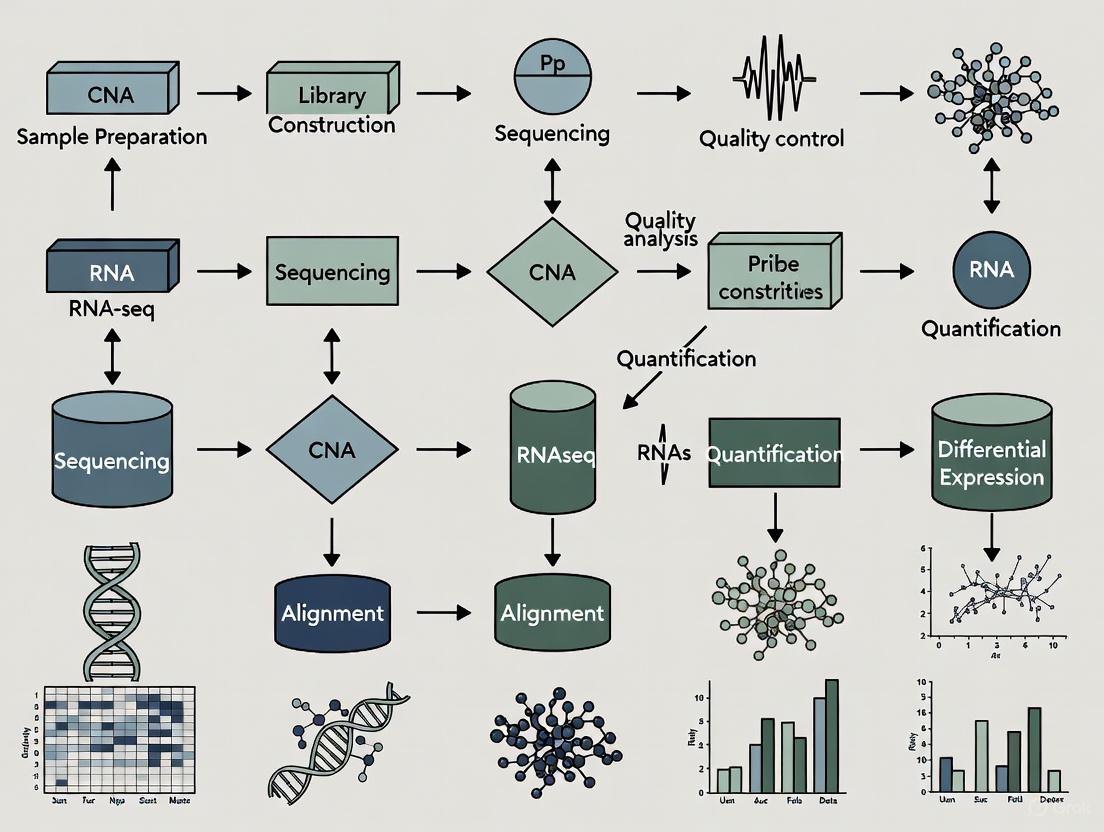
Figure 1: RNA-seq Bioinformatics Workflow

Quality Control and Trimming: Initial quality assessment of raw sequencing reads is crucial for detecting sequencing errors, contaminants, and PCR artifacts [10] [9]. Tools such as FastQC provide comprehensive quality metrics, while trimming tools like fastp or Trim Galore remove adapter sequences and low-quality bases to improve mapping rates [10]. Key parameters to assess include sequence quality, GC content, adapter content, overrepresented k-mers, and duplicated reads [9].

Read Alignment: Three primary strategies exist for aligning processed reads [9]:

• Genome Mapping: Aligning reads to a reference genome using splice-aware aligners (e.g., STAR, HISAT2)
• Transcriptome Mapping: Direct alignment to reference transcript sequences
• De Novo Assembly: Reconstructing transcripts without a reference genome using tools like Trinity

The choice of strategy depends on reference genome availability and quality, with genome-based approaches generally preferred when high-quality references exist [9].

Transcript Quantification: This step estimates gene and transcript expression levels from aligned reads [15] [9]. Tools like RSEM (RNA-Seq by Expectation Maximization) and kallisto account for multi-mapping reads (those that align to multiple genomic locations) and allocate them probabilistically among transcripts [15]. RSEM is particularly notable as it can work with or without a reference genome, making it valuable for non-model organisms [15]. For accurate quantification, it's essential to use methods that properly handle ambiguously-mapping reads rather than simply discarding them [15].

Table 2: Quantitative Comparison of Differential Expression Tools

Tool	Statistical Distribution	Normalization Method	Replicates Required	Best Use Case
DESeq2	Negative Binomial	Median of ratios	Recommended	Standard DE analysis with biological replicates
edgeR	Negative Binomial	TMM, RLE	Required	Experiments with small sample sizes
limma-voom	Log-Normal	TMM	Recommended	Complex experimental designs
Cufflinks	Poisson	FPKM	Not required	Isoform-level differential expression
SAMseq	Non-parametric	Internal	Recommended	Data not fitting standard distributions

Differential Expression Analysis: This final analytical step identifies genes with statistically significant expression changes between conditions [13]. The choice of tool depends on experimental design, replication, and data characteristics. DESeq2 and edgeR are widely used methods that employ negative binomial distributions to model count data and account for biological variability [13]. Both tools require raw count data as input and perform their own normalization procedures to correct for library size and composition biases [13].

Functional Profiling: The final step typically involves biological interpretation of differential expression results through functional enrichment analysis [9]. Tools for Gene Ontology analysis, pathway enrichment (KEGG, Reactome), and network analysis help place the molecular changes in biological context, identifying affected processes, pathways, and functions.

Research Reagent Solutions and Materials

Table 3: Essential Research Reagents and Materials for RNA-seq

Reagent/Material	Function	Examples/Specifications
RNA Stabilization Reagents	Preserve RNA integrity immediately after sample collection	RNAlater, TRIzol, PAXgene
Poly(A) Selection Beads	Enrich for polyadenylated mRNA	Oligo(dT) magnetic beads
RNA Fragmentation Reagents	Fragment RNA to appropriate size for sequencing	Metal cations, heat, enzymatic fragmentation
Reverse Transcriptase	Synthesize cDNA from RNA templates	SuperScript IV, Maxima H-minus
Library Preparation Kits	Prepare sequencing libraries with adaptors	Illumina TruSeq, NEB Next Ultra II
cDNA Synthesis Kits	Generate cDNA for long-read sequencing	PacBio SMRTbell, ONT cDNA
Spike-in RNA Controls	Normalization and quality control	ERCC RNA Spike-In Mix, SIRV sets
Quality Control Assays	Assess RNA and library quality	Bioanalyzer, TapeStation, Qubit

Advanced Considerations and Recent Developments

Long-Read RNA Sequencing Technologies

Recent advances in long-read RNA sequencing (lrRNA-seq) technologies have transformed transcriptome analysis by enabling full-length transcript sequencing [12]. The Long-read RNA-Seq Genome Annotation Assessment Project (LRGASP) Consortium systematically evaluated these methods, revealing that libraries with longer, more accurate sequences produce more accurate transcripts than those with increased read depth, while greater read depth improved quantification accuracy [12].

Key findings from lrRNA-seq assessments include:

• cDNA-PacBio and R2C2-ONT datasets produce the longest read-length distributions
• Sequence quality is higher for CapTrap-PacBio, cDNA-PacBio and R2C2-ONT than other approaches
• For well-annotated genomes, reference-based tools demonstrate the best performance
• Incorporating orthogonal data and replicate samples is advised for detecting rare and novel transcripts

Experimental Design Considerations

Proper experimental design is crucial for robust differential expression analysis. Key considerations include:

Replication:

• Biological replicates (different biological units) are essential for capturing natural variation
• Technical replicates (same sample processed multiple times) help assess technical noise
• Minimum 3 biological replicates per condition recommended, with more for subtle effects

Sequencing Depth:

• Balance between sufficient depth for detection and cost considerations
• Typically 20-50 million reads per sample for standard differential expression in mammalian genomes
• Increased depth required for detecting low-abundance transcripts or complex isoforms

Batch Effects:

• Distribute experimental conditions across sequencing batches
• Randomize processing order to avoid confounding technical and biological variation
• Use statistical methods like COMBAT or ARSyN to correct for batch effects when unavoidable

Method Selection and Benchmarking

With numerous available tools for each step of RNA-seq analysis, selection of appropriate methods is challenging. Recent benchmarking studies provide guidance:

• For differential expression, DESeq2, edgeR, and limma-voom generally show good performance [13]
• For transcript quantification, methods like RSEM that properly handle multi-mapping reads outperform simple count-based approaches [15]
• Performance of analytical tools can vary across species, suggesting that optimization for specific organisms may be necessary [10]
• For alternative splicing analysis, rMATS demonstrates good performance for detecting differentially spliced isoforms [10]

RNA-seq has fundamentally transformed transcriptomics by providing an unprecedented detailed view of transcriptomes. Understanding the core concepts of transcriptomes, sequencing reads, and differential expression analysis is essential for designing, executing, and interpreting RNA-seq experiments effectively. The continuous development of both experimental protocols and computational methods ensures that RNA-seq will remain a cornerstone technology for biological discovery and translational research, particularly in drug development where understanding gene expression changes is critical for target identification, mechanism elucidation, and biomarker discovery.

As the field evolves, integration of long-read technologies, single-cell approaches, and multi-omics frameworks will further enhance our ability to address the central question of differential expression across diverse biological contexts and experimental conditions.

RNA sequencing (RNA-Seq) has revolutionized transcriptomic research, providing a powerful tool for large-scale inspection of mRNA levels in living cells [16]. This application note outlines the complete end-to-end RNA-Seq data analysis workflow, from raw sequencing data to biological interpretation. The protocol is designed to enable researchers and drug development professionals to perform differential gene expression analysis, gaining critical insights into gene function and regulation that can inform therapeutic development and biomarker discovery.

Experimental Design and Data Acquisition

A successful RNA-Seq study begins with a well-considered experimental design that ensures the generated data can answer the biological questions of interest [17]. Key considerations include:

• RNA Extraction Protocol: Choose between poly(A) selection for mRNA enrichment or ribosomal RNA (rRNA) depletion. Poly(A) selection requires high-quality RNA with minimal degradation, while ribosomal depletion is suitable for lower-quality samples or bacterial studies where mRNA lacks polyadenylation [17].
• Library Strandedness: Strand-specific protocols preserve information about the originating DNA strand, crucial for analyzing antisense or overlapping transcripts [17].
• Sequencing Configuration: Paired-end reads are preferable for de novo transcript discovery or isoform expression analysis, while single-end reads may suffice for gene expression studies in well-annotated organisms [17].
• Sequencing Depth: Deeper sequencing (more reads) enables detection of more transcripts and improves quantification precision, particularly for lowly-expressed genes. Requirements vary from as few as 5 million mapped reads for medium-highly expressed genes to 100 million reads for comprehensive transcriptome coverage [17].
• Replication: The number of biological replicates depends on technical variability, biological variability, and desired statistical power for detecting differential expression [17].

Table 1: Key Experimental Design Decisions in RNA-Seq

Design Factor	Options	Considerations
RNA Selection	Poly(A) enrichment	Requires high RNA integrity; captures only polyadenylated transcripts
	rRNA depletion	Works with degraded samples (e.g., FFPE); captures non-polyadenylated RNA
Library Type	Strand-specific	Preserves strand information; identifies antisense transcripts
	Non-stranded	Standard approach; lower cost
Sequencing Type	Single-end	Cost-effective; sufficient for basic expression quantification
	Paired-end	Better for isoform analysis, novel transcript discovery
Read Length	50-300 bp	Longer reads improve mappability, especially across splice junctions

Computational Analysis Workflow

The computational analysis of RNA-Seq data transforms raw sequencing files into interpretable biological results through a multi-step process.

From Raw Reads to Read Counts

Quality Control of Raw Reads Initial quality assessment checks sequence quality, GC content, adapter contamination, overrepresented k-mers, and duplicated reads to identify sequencing errors or PCR artifacts [17]. FastQC is commonly used for this analysis [17] [16]. Trimmomatic or the FASTX-Toolkit can remove low-quality bases and adapter sequences [17] [16].

Read Alignment Processed reads are aligned to a reference genome or transcriptome using tools such as HISAT2, STAR, or TopHat2 [16] [18]. Alignment quality metrics include the percentage of mapped reads (expected 70-90% for human genome), read coverage uniformity across exons, and strand specificity [17]. The output is typically in SAM/BAM format [19].

Quantification Aligned reads are assigned to genomic features (genes, transcripts) using quantification tools like featureCounts or HTSeq [16] [18]. This generates a count matrix where each value represents the number of reads unambiguously assigned to a specific gene in a particular sample [19]. It is crucial that these values represent raw counts, not normalized values, for subsequent statistical analysis [19].

Differential Expression Analysis

Data Normalization and Modeling Count matrices are imported into statistical environments such as R/Bioconductor for differential expression analysis [19]. Methods like DESeq2, edgeR, or limma-voom employ specific normalization approaches to account for differences in library size and RNA composition, then model expression data using statistical distributions (typically the negative binomial distribution for count data) [19].

Statistical Testing and Results Extraction These tools test each gene for statistically significant differences in expression between experimental conditions, generating measures of effect size (fold change) and significance (p-value, adjusted p-value) [19]. Results can be visualized through MA-plots, volcano plots, and heatmaps to identify patterns of differential expression [16].

Workflow Visualization

The Scientist's Toolkit: Essential Research Reagents and Software

Table 2: Essential Tools for RNA-Seq Data Analysis

Tool Name	Category	Primary Function	Application Notes
FastQC	Quality Control	Assesses raw read quality	Identifies sequencing errors, adapter contamination, GC biases [17] [16]
Trimmomatic	Preprocessing	Trims adapters, low-quality bases	Improves mappability by removing poor sequence ends [17] [16]
HISAT2	Alignment	Aligns reads to reference genome	Efficient for splice-aware alignment; faster than earlier tools [16]
STAR	Alignment	Aligns reads to reference genome	Excellent for detecting splice junctions; higher resource requirements [19]
featureCounts	Quantification	Assigns reads to genomic features	Generates count matrix from aligned reads [16]
DESeq2	Differential Expression	Identifies differentially expressed genes	Uses negative binomial model; robust for experiments with limited replicates [19]
edgeR	Differential Expression	Identifies differentially expressed genes	Similar statistical model to DESeq2; different normalization approaches [19] [18]
R/Bioconductor	Analysis Environment	Statistical analysis and visualization	Comprehensive ecosystem for genomic data analysis [19]
8-Ethyl Irinotecan	8-Ethyl Irinotecan, CAS:947687-02-7, MF:C35H42N4O6, MW:614.7 g/mol	Chemical Reagent	Bench Chemicals
Itopride N-Oxide	Itopride N-Oxide Reference Standard|141996-98-7	Itopride N-Oxide (CAS 141996-98-7) is a key metabolite and impurity standard for pharmaceutical research. For Research Use Only. Not for human use.	Bench Chemicals

Quality Control Checkpoints

Robust RNA-Seq analysis requires quality assessment at multiple stages to ensure data integrity and reliability of conclusions [17].

Post-Alignment QC After read alignment, tools like Picard, RSeQC, or Qualimap assess mapping statistics, including the percentage of mapped reads, uniformity of exon coverage, and detection of 3' bias (indicative of RNA degradation) [17]. For mammalian genomes, 70-90% of reads should typically map to the reference [17].

Post-Quantification QC Following transcript quantification, checks for GC content and gene length biases inform appropriate normalization methods [17]. For well-annotated genomes, analyzing the biotype composition of the sample (e.g., mRNA vs. rRNA content) provides insights into RNA purification efficiency [17].

Batch Effect Mitigation Technical variability from different sequencing runs, library preparation dates, or personnel should be minimized through experimental design [18]. When processing samples in batches, include controls in each batch and randomize sample processing [17].

Advanced Analysis and Interpretation

Exploratory Data Analysis Prior to formal differential expression testing, exploratory data analysis techniques such as Principal Component Analysis (PCA) visualize overall data structure, assessing sample similarity and identifying potential outliers [18]. PCA reduces the high-dimensional gene expression data to two or three dimensions that capture the greatest variance, allowing assessment of whether intergroup differences exceed intragroup variability [18].

Functional Enrichment Analysis Differentially expressed genes can be further analyzed for enrichment of biological pathways, Gene Ontology (GO) terms, or other functional annotations [18]. This moves beyond individual gene lists to identify biological processes, molecular functions, and cellular compartments that are statistically overrepresented among the differentially expressed genes.

Data Visualization Effective visualization techniques enhance interpretation of RNA-Seq results:

• Heatmaps: Display expression patterns of significant genes across samples, often with clustering to identify co-expressed genes [16].
• Volcano Plots: Visualize the relationship between statistical significance (p-value) and magnitude of change (fold change) for all tested genes [16].
• MA-Plots: Show the relationship between average expression intensity and fold change, highlighting potential biases [19].

A comprehensive understanding of the end-to-end RNA-Seq workflow empowers researchers to design robust experiments, implement appropriate analysis strategies, and accurately interpret results. This structured approach from experimental design through functional interpretation ensures maximum biological insight from transcriptomic datasets, supporting drug development and basic research applications. As RNA-Seq methodologies continue to evolve, maintaining this "big picture" perspective enables researchers to adapt new computational methods while maintaining rigorous analytical standards.

Within the broader context of RNA sequencing (RNA-seq) data analysis workflow research, a thorough understanding of the core file formats is fundamental. The journey from raw sequencing data to biological insight is codified in a series of specialized files, each representing a distinct stage of processing and abstraction. This guide decodes three essential formats—FASTQ, BAM, and Count Matrices—detailing their structures, roles in the analytical pipeline, and the practical protocols for working with them. Mastery of these formats empowers researchers and drug development professionals to execute robust, reproducible transcriptomic analyses, forming the computational bedrock for advancements in molecular biology and personalized medicine [20].

RNA sequencing has revolutionized transcriptomics by enabling genome-wide quantification of RNA abundance with high resolution and accuracy [20]. The transformation of a biological sample into interpretable gene expression data is a multi-stage computational process. Each stage produces a characteristic file format that encapsulates specific information:

• FASTQ files represent the raw output of sequencing instruments, containing the nucleotide sequences and their associated quality scores.
• BAM files contain the aligned sequences, representing where these reads map within a reference genome or transcriptome.
• Count Matrices are the final, summarized quantitative data, aggregating reads to estimate gene or transcript expression levels for each sample in an experiment.

This progression from raw sequences to a numerical matrix is critical for downstream statistical analysis, including the identification of differentially expressed genes (DEGs) [20]. The following workflow diagram illustrates the relationship between these core file formats and the key processing steps.

The File Formats: Structures and Functions

FASTQ: The Raw Sequencing Read Format

Function: The FASTQ format is the primary output of next-generation sequencing (NGS) platforms. It stores the nucleotide sequences (reads) generated by the sequencer and, crucially, the per-base quality scores that indicate the confidence of each base call [21] [20]. This quality information is vital for assessing sequencing run success and for preprocessing.

Structure: Each sequence in a FASTQ file is represented by four lines:

• Line 1 (Sequence Identifier): Begins with an @ character and contains information about the sequencing instrument and run.
• Line 2 (Raw Sequence Letters): The actual nucleotide sequence (A, C, G, T, N).
• Line 3 (Separator): A + character, sometimes followed by the same identifier as line 1.
• Line 4 (Quality Scores): A string of characters encoding the per-base Phred quality score, indicating the probability of a base call error.

Table: Key Characteristics of the FASTQ Format

Characteristic	Description	Role in Analysis
Primary Content	Nucleotide sequences (reads)	Represents fragments of the transcriptome present in the sample.
Quality Scores	Per-base Phred score (ASCII encoded)	Enables quality control; identifies low-quality bases for trimming.
File Size	Very large (often gigabytes)	Requires significant storage and computational resources.
Data Type	Raw, unprocessed data	The starting point for all downstream analysis.

BAM/SAM: The Aligned Sequence Format

Function: The BAM (Binary Alignment/Map) file, and its text-based equivalent SAM, store the alignment information of sequencing reads to a reference genome or transcriptome. This step identifies the genomic origin of each RNA fragment, allowing researchers to determine which genes are being expressed [20]. The BAM format is binary, making it compressed and efficient for storage and indexing, whereas SAM is human-readable.

Structure: A BAM file consists of a header section and an alignment section.

• Header: Contains metadata about the reference sequence, the alignment program used, and the sorting order.
• Alignment Section: Each line represents a single read, containing key information such as the reference sequence name, mapping position, mapping quality (MAPQ), and the CIGAR string that details the alignment (e.g., matches, insertions, deletions).

Table: Key Characteristics of the BAM/SAM Format

Characteristic	Description	Role in Analysis
Primary Content	Alignment coordinates of reads	Locates transcribed fragments within the genome.
Mapping Quality	Per-read confidence in alignment	Allows filtering of poorly or ambiguously mapped reads.
CIGAR String	Compact string representing alignment	Details matches, mismatches, insertions, and deletions.
Binary vs. Text	BAM is compressed binary; SAM is text	BAM saves disk space and is faster to process.

Count Matrix: The Gene Expression Quantification Format

Function: The count matrix is the final product of the data preprocessing pipeline and the direct input for differential expression analysis. It is a table that summarizes the number of sequencing reads assigned to each genomic feature (e.g., gene, transcript) for every sample in the study [20]. These "raw counts" are used by statistical tools like DESeq2 to identify genes that are significantly differentially expressed between conditions.

Structure: A count matrix is a two-dimensional table where:

• Rows represent genomic features (genes or transcripts).
• Columns represent individual samples or libraries.
• Cells contain integer values representing the number of reads that mapped to that feature in that sample.

Table: Example Structure of a Gene Count Matrix

Gene	Sample1Control	Sample2Control	Sample3Treated	Sample4Treated
Gene_A	150	165	2050	2100
Gene_B	50	45	55	60
Gene_C	2000	1800	100	150

Experimental Protocols for Data Processing

Protocol 1: From FASTQ to BAM - Read Alignment

This protocol covers the critical steps of quality control and alignment to convert raw sequencing data into aligned BAM files [21] [20].

Step 0: Software Installation

• Install the necessary bioinformatics tools using a package manager like Conda to ensure version control and reproducibility.
• Example Command:

Step 1: Quality Control of Raw FASTQ Files

• Objective: Assess sequencing quality and identify potential issues like adapter contamination or low-quality bases.
• Method: Use FastQC to generate a quality report. Visually inspect the HTML output for warnings in modules like "Per Base Sequence Quality" and "Adapter Content" [21].
• Example Command:

Step 2: Trimming and Adapter Removal

• Objective: Clean the reads by removing adapter sequences, overrepresented sequences, and low-quality bases.
• Method: Use Trimmomatic or a similar tool. Parameters must be set to balance data quality with retention of sufficient read length.
• Example Command:

Step 3: Read Alignment to a Reference Genome

• Objective: Map each cleaned sequencing read to its correct location in the reference genome.
• Method: Use an aligner such as HISAT2 (commonly used for RNA-seq) or STAR. First, download and index the reference genome for the organism of study.
• Example Commands:

Step 4: SAM to BAM Conversion and Sorting

• Objective: Convert the human-readable SAM file to a compressed BAM file and sort it by genomic coordinate for efficient downstream analysis.
• Method: Use samtools, a ubiquitous toolkit for handling aligned sequencing data.
• Example Commands:

Protocol 2: From BAM to Count Matrix - Read Quantification

This protocol details the process of generating a gene-level count matrix from sorted BAM files, which is ready for statistical analysis [21] [20].

Step 1: Post-Alignment Quality Control

• Objective: Verify the quality of the alignments and identify any issues like high rates of multi-mapping reads.
• Method: Use tools like Qualimap or samtools stats to generate alignment statistics, including the percentage of uniquely mapped reads.

Step 2: Read Quantification with featureCounts

• Objective: Count the number of reads mapped to each gene.
• Method: Use featureCounts (from the Subread package) or HTSeq-count. These tools take the aligned BAM file and a reference annotation file (GTF/GFF) that defines the genomic coordinates of genes.
• Example Command:
  • -T 4: Use 4 threads for computation.
  • -p: Count fragments (for paired-end data) instead of reads.
  • -a annotation.gtf: Specify the file with gene annotations.
  • -o gene_counts.txt: Specify the output file.

Step 3: Consolidating the Count Matrix

• Objective: Combine the output from multiple samples into a single count matrix for downstream analysis in R or Python.
• Method: The output of featureCounts is a text file. The count columns for all samples can be merged using custom scripts in R or Python, ensuring the rows (genes) are consistent across samples. The final matrix should look like the example in Section 2.3.

The following diagram visualizes the complete computational workflow from FASTQ files to a count matrix, incorporating the key steps from both protocols.

The Scientist's Toolkit: Essential Research Reagents & Software Solutions

The computational pipeline for RNA-seq data processing relies on a suite of software tools, each functioning as a critical "research reagent" to transform data from one format to the next.

Table: Essential Computational Tools for RNA-seq Analysis

Tool / 'Reagent'	Function	Key Input	Key Output
FastQC [21]	Quality control check of raw sequencing data.	FASTQ file	HTML report with quality metrics
Trimmomatic [21]	Removes adapter sequences and low-quality bases.	Raw FASTQ file	Cleaned/Trimmed FASTQ file
HISAT2 [21] [20]	Aligns RNA-seq reads to a reference genome.	Cleaned FASTQ file, Reference genome	SAM file
STAR [20]	Alternative, splice-aware aligner.	Cleaned FASTQ file, Reference genome	SAM file
Samtools [21] [20]	Manipulates alignments; converts, sorts, and indexes BAM files.	SAM/BAM file	Sorted, indexed BAM file
featureCounts [21] [20]	Quantifies reads mapped to genomic features.	Sorted BAM file, Annotation file (GTF)	Count matrix (text file)
R/Bioconductor (DESeq2) [21]	Performs statistical analysis for differential expression.	Count matrix	List of differentially expressed genes
Ambroxol	Ambroxol Hydrochloride		Bench Chemicals
(S)-Indacaterol	(S)-Indacaterol	(S)-Indacaterol is a long-acting beta-2 adrenoceptor agonist (LABA) for COPD research. This product is for research use only (RUO).	Bench Chemicals

Robust RNA sequencing data is foundational to transcriptomic research, yet the biological conclusions drawn from an experiment are only as reliable as its initial design. Thoughtful experimental design is critical to ensure high-quality data and interpretable results, as no amount of statistical sophistication can separate confounded factors after data collection [22] [18]. This document outlines comprehensive protocols and application notes for key considerations in RNA-seq experimental design, including replication strategy, sequencing depth optimization, and library preparation selection, framed within the broader context of RNA-seq data analysis workflow research. These guidelines are essential for researchers, scientists, and drug development professionals seeking to generate biologically meaningful transcriptomic data.

Experimental Design Considerations

The Critical Importance of Replication

Biological replicates—different biological samples representing the same condition—are absolutely essential for differential expression analysis as they allow measurement of the biological variation within a population [23]. The variation between biological replicates is typically greater than technical variation, and biological replication simultaneously counteracts random technical variation through independent sample preparation [24].

Protocol: Implementing Proper Replication Strategy

• Minimum Replicates: Include a minimum of 3 biological replicates per condition, though 5-6 is ideal for robust statistical power [25] [23].
• Cell Line Considerations: For cell line experiments, prepare replicates as independently as possible using different frozen cell stocks, freshly prepared media, and different growth factor batches [23].
• Pooling Strategy: If pooling is unavoidable due to material limitations, pool the same number of individuals for each condition and ensure pooled individuals are similar in sex, age, and other relevant factors. Each pooled set counts as a single replicate [23].

Table 1: Impact of Replication on Differential Expression Detection

Replication Strategy	Statistical Power	Ability to Estimate Biological Variance	Cost Efficiency
2 Biological Replicates	Low	Limited	Moderate
3-5 Biological Replicates	Good	Adequate	High
>5 Biological Replicates	Excellent	Robust	Lower
Technical Replicates Only	Very Low	None	Low

Sequencing Depth Guidelines

Sequencing depth requirements vary significantly based on the specific research objectives and experimental questions. Generally, spending resources on more biological replicates provides better returns than increasing sequencing depth [23].

Protocol: Determining Optimal Sequencing Depth

• General Gene-Level Differential Expression: 15 million single-end reads per sample is often sufficient with good replication (>3 replicates). ENCODE guidelines suggest 30 million SE reads per sample (stranded) [23].
• Detection of Lowly-Expressed Genes: Sequence deeper with at least 30-60 million reads depending on the level of expression desired, starting with 30 million with adequate replication [23].
• Isoform-Level Analysis: For known isoforms, use at least 30 million paired-end reads per sample; for novel isoform discovery, use >60 million reads per sample [23].

Table 2: Sequencing Depth Recommendations by Experimental Goal

Experimental Goal	Recommended Depth	Read Type	Key Considerations
Gene-level DE	15-30 million reads	SE or PE ≥50bp	More replicates preferred over depth
Low-expression DE	30-60 million reads	PE ≥50bp	Balance depth with replication
Isoform-level (known)	≥30 million reads	PE ≥50bp	Longer reads better for junctions
Isoform-level (novel)	>60 million reads	PE ≥50bp	Careful RNA QC essential
3' mRNA-Seq (QuantSeq)	1-5 million reads	SE or PE	Cost-effective for large screens

Library Preparation Selection

The choice between whole transcriptome and 3' mRNA-seq approaches significantly impacts the information content, cost structure, and analytical requirements of an RNA-seq experiment [26].

Protocol: Selecting Library Preparation Method

Choose Whole Transcriptome/Total RNA-Seq if you need:

• A global view of all RNA types (coding and non-coding)
• Information about alternative splicing, novel isoforms, or fusion genes
• To work with samples where the poly(A) tail might be absent or highly degraded (e.g., prokaryotic RNA, some clinical samples) [26]

Choose 3' mRNA-Seq (e.g., QuantSeq) if you need:

• Accurate and cost-effective gene expression quantification
• High-throughput screening of many samples
• A streamlined workflow with simpler data analysis
• To efficiently profile mRNA expression from degraded RNA and challenging sample types (like FFPE) [26]

Managing Technical Variation and Batch Effects

Technical variation in RNA-seq experiments stems from multiple sources, including differences in RNA quality/quantity, library preparation batch effects, flow cell and lane effects, and adapter bias [22]. Library preparation has been identified as the largest source of technical variation [22].

Protocol: Minimizing Batch Effects

• Randomization: Randomize samples during preparation and dilute to the same concentration [22].
• Multiplexing: Index and multiplex samples across all sequencing lanes/flow cells when possible [22].
• Blocking Design: When complete multiplexing isn't possible, use a blocking design that includes samples from each experimental group on each sequencing lane [22] [23].
• Metadata Collection: Meticulously record all potential batch effect sources (RNA isolation date, library prep date, researcher, reagents) for inclusion in statistical models [23].

Checklist for Identifying Batches

• Were all RNA isolations performed on the same day?
• Were all library preparations performed on the same day?
• Did the same person perform the RNA isolation/library preparation for all samples?
• Were the same reagents used for all samples?
• Was the RNA isolation/library preparation performed in the same location?
• If any answer is 'No', then batches exist and should be accounted for in experimental design and analysis [23].

The Scientist's Toolkit: Research Reagent Solutions

Table 3: Essential Materials for RNA-seq Experiments

Reagent/Kit	Function	Application Notes
Poly(A) Selection Kits (e.g., NEBNext)	Enriches for mRNA by selecting polyadenylated transcripts	Standard for mRNA sequencing; misses non-polyadenylated RNAs
RiboMinus Kits	Depletes ribosomal RNA from total RNA	Preserves non-coding and non-polyadenylated RNAs
RiboZero Kits	Depletes ribosomal RNA from total RNA	Alternative ribosomal depletion method
Ultralow DR Library Kit	Library preparation for low input samples	Essential for limited clinical or sorted cell samples
QuantSeq 3' mRNA-Seq Kit	3' focused library preparation	Ideal for high-throughput quantitative studies
Stranded mRNA-Seq Kit	Maintains strand information in library prep	Important for identifying antisense transcription
SPIA Amplification	Linear amplification of cDNA	Critical for low input samples to obtain sufficient material
Promethazine-d4	Promethazine-d4 Stable Isotope	Promethazine-d4 is a deuterated internal standard for accurate LC-MS/MS research. For Research Use Only. Not for human or veterinary use.
4-Pyridoxic Acid-d3	4-Pyridoxic Acid-d3, MF:C8H9NO4, MW:186.18 g/mol	Chemical Reagent

Comparative Analysis of Library Preparation Methods

Protocol: Performance Characteristics of WTS vs. 3' mRNA-Seq

A comparative study analyzing murine livers following normal or high iron diets demonstrated that both whole transcriptome and 3' mRNA-seq methods generate highly similar biological conclusions despite technical differences [26].

Key Findings:

• Whole Transcriptome Sequencing: Detects more differentially expressed genes and assigns more reads to longer transcripts, requiring stringent length normalization [26].
• 3' mRNA-Seq: Better detects short transcripts and provides more equal coverage across transcripts regardless of length, with simpler normalization requirements [26].
• Concordance: Both methods show high reproducibility between biological replicates and identify the same key biological pathways, though with some ranking differences in secondary pathways [26].

Practical Implementation Considerations:

• For 3' mRNA-Seq, ensure well-curated 3' annotation is available, especially for non-model organisms [26].
• Whole transcriptome sequencing requires careful quality control of RNA quality, particularly restricting analysis to high RIN samples when performing isoform-level analysis [23].

Proper experimental design remains the most critical factor in generating meaningful RNA-seq data. By carefully considering replication strategy, sequencing depth, library preparation methods, and batch effect management during the planning stages, researchers can ensure their experiments yield biologically interpretable results with minimal technical artifacts. The protocols and guidelines presented here provide a framework for designing robust RNA-seq experiments that effectively address specific research questions while optimizing resource allocation in both academic and drug development contexts.

From Raw Reads to Results: A Practical Walkthrough of the Analysis Pipeline

In RNA sequencing (RNA-seq) analysis, the initial quality control (QC) step is crucial for assessing the quality of raw sequencing data before proceeding with downstream analyses. High-throughput sequencing pipelines generate tremendous amounts of data that cannot be meaningfully interpreted without proper QC checks to identify potential issues that might compromise biological conclusions [27] [18]. Effective QC allows researchers to detect problems early, including sequencing errors, adapter contamination, or biases introduced during library preparation, thereby saving substantial time and effort in subsequent analysis stages.

The standard tool for initial QC assessment is FastQC, which provides a comprehensive evaluation of raw sequence data in FASTQ format. Following individual FastQC runs, MultiQC aggregates results from multiple samples and various bioinformatics tools into a single interactive report, enabling efficient comparison of QC metrics across all samples in an experiment [28] [29]. This combined approach provides researchers with a powerful framework for quality assessment, ensuring that only high-quality data progresses through the RNA-seq workflow, ultimately leading to more reliable and reproducible results in transcriptomic studies and drug development research.

Theoretical Foundation and Key Metrics

Understanding FASTQ Format and Sequencing Quality

RNA-seq data typically begins in FASTQ format, which stores called bases along with corresponding quality scores for each sequencing read [27]. The quality scores, expressed as Phred-scale values (Q), represent the probability of an incorrect base call. For example, Q30 denotes a 99.9% base call accuracy (1 error in 1,000 bases), and high-quality data should typically have over 80% of bases with Q30 or higher [27]. FastQC evaluates multiple aspects of this raw sequence data, generating metrics that help researchers identify potential issues before proceeding with alignment and quantification.

Critical Quality Control Metrics

FastQC examines several key metrics that provide insights into data quality. The per-base sequence quality assesses how quality scores change across read positions, typically showing a slight quality reduction toward read ends [27]. The adapter content metric identifies the presence of adapter sequences, which must be trimmed before alignment [27]. GC content evaluation checks whether the distribution of G and C nucleotides matches the expected organism-specific composition, while sequence duplication levels help identify potential technical duplicates or highly expressed transcripts [30] [29]. For RNA-seq data, some duplication is expected due to varying transcript abundances, but excessive duplication may indicate low library complexity or over-amplification [30] [29]. Understanding these metrics is essential for correctly interpreting FastQC reports and making informed decisions about data processing.

Materials and Reagent Solutions

Research Reagent Solutions

Table 1: Essential tools and materials for RNA-seq quality control

Item	Function	Specifications
FastQC	Quality control tool for raw sequencing data	Analyzes FASTQ files; provides metrics on quality scores, GC content, adapter contamination, sequence duplication [31] [27]
MultiQC	Aggregate QC reports	Summarizes results from FastQC and other tools across multiple samples into a single HTML report [28] [29]
RNA-seq Data	Input raw sequencing files	Typically in FASTQ format (compressed: .fastq.gz); contains sequence reads and quality scores [27]
Computing Resources	Hardware for analysis	Linux environment; ≥32GB RAM for larger genomes; ≥1TB storage; grid cluster for parallel processing [27]

Experimental Protocol and Workflow

The following diagram illustrates the comprehensive quality control workflow for RNA-seq data, from raw sequencing reads to aggregated quality assessment:

FastQC Analysis Protocol

Step 1: Load Required Modules and Run FastQC On a computing cluster with bioinformatics tools pre-installed, begin by loading necessary modules and executing FastQC:

The -o parameter specifies the output directory for FastQC results. FastQC can process BAM, SAM, or FASTQ files in any variant, making it versatile for different stages of RNA-seq analysis [31].

Step 2: Run FastQC on Multiple Samples For studies with multiple samples, process all files efficiently:

This generates individual HTML reports and ZIP files for each sample, containing comprehensive metrics on sequence quality [31].

MultiQC Aggregation Protocol

Step 3: Aggregate Results with MultiQC After generating individual FastQC reports, compile them into a comprehensive summary:

MultiQC automatically scans the specified directory for recognized log files (including FastQC outputs) and generates an interactive HTML report aggregating statistics across all samples [31] [28]. The -n parameter allows custom naming of the output file.

Step 4: Transfer and View Reports For researchers using remote servers, transfer the report to a local machine for viewing:

The HTML report can then be downloaded using file transfer tools like FileZilla and opened in a web browser for interactive exploration of the results [30] [28].

Results Interpretation and Quality Assessment

Interpretation Framework for QC Metrics

The following diagram illustrates the decision-making process for evaluating key QC metrics and determining appropriate actions:

Key Metrics and Acceptance Criteria

Table 2: FastQC metric interpretation guidelines for RNA-seq data

Metric	Optimal Result	Warning Signs	Potential Causes	Action Required
Per-Base Sequence Quality	Quality scores mostly in green zone (>Q28); minimal decrease at read ends [27]	Scores drop below Q20 (orange/red); significant quality decrease at ends	Sequencing chemistry degradation; poor cluster detection	Proceed with trimming of low-quality bases [27]
Adapter Content	<1% adapter contamination across all positions [27]	>5% adapter content, especially at read ends	Short insert sizes; adapter dimer contamination	Trim adapter sequences before alignment [27]
GC Content	Approximately organism-specific % (e.g., ~40-60% for mouse/human); normal distribution shape [29]	Bimodal distribution; significant deviation from expected %	Contamination; sequencing artifacts; library preparation bias	Investigate potential contamination sources [29]
Sequence Duplication	Moderate duplication expected for highly expressed genes [30]	>50% duplication in non-ribosomal reads	Low library complexity; PCR over-amplification; insufficient sequencing depth	Evaluate library preparation; consider increasing sequencing depth [30]

MultiQC Report Navigation

The MultiQC report provides an interactive interface for comparing samples. The "General Statistics" table offers a quick overview of key metrics across all samples, including total sequences, percentage of duplicates, and overall mean quality scores [28] [29]. Configure columns using the "Configure Columns" button to display the most relevant metrics for your experiment. The toolbox on the right enables sample highlighting, renaming, and plot customization for enhanced data exploration and presentation [28].

Status checks are color-coded: green (PASS), orange (WARN), and red (FAIL). For RNA-seq data, some warnings may be expected due to the nature of transcriptomic data, such as sequence duplication from highly expressed genes [30]. The end of the report contains a heatmap summary of all modules, providing a rapid visual assessment of potential problem areas across samples [28].

Troubleshooting and Technical Notes

Common Issues and Solutions

• High adapter content: This indicates that a significant proportion of reads contain adapter sequences, requiring trimming before alignment. Use tools like Trimmomatic with appropriate adapter files [27].
• Low-quality scores: Poor quality, particularly at the 3' end of reads, may necessitate more stringent quality trimming. Re-run FastQC after trimming to verify improvement [27].
• Abnormal GC content: Unexpected GC distributions may indicate contamination or technical artifacts. Compare with expected organism-specific GC content and investigate potential sources of contamination [29].
• High duplication levels: While some duplication is normal in RNA-seq due to highly expressed transcripts, excessive duplication may indicate low library complexity. Consider whether the sequencing depth is sufficient for your experimental goals [30] [29].

Installation and Implementation Notes

MultiQC can be installed through multiple package managers: pip install multiqc for PyPI, conda install multiqc for Conda, or via Docker/Singularity containers for reproducible environments [32]. When running MultiQC on a computing cluster, ensure all output files from various tools (FastQC, STAR, etc.) are accessible in the directory structure for comprehensive aggregation [31] [29]. For large studies with multiple analysis steps, MultiQC can incorporate outputs from alignment tools (e.g., STAR), quantification tools (e.g., featureCounts), and others, providing a complete overview of the entire RNA-seq workflow [31] [29].

When interpreting results, researchers should consider that some FastQC warnings may be expected for specific RNA-seq protocols. For example, uneven coverage or sequence duplication is common in transcriptomic data due to varying transcript abundance [30]. The critical assessment involves comparing metrics across all samples to identify outliers rather than focusing solely on absolute values of individual samples.

Within the comprehensive workflow of RNA-seq data analysis, the step of trimming and adapter removal is a critical preprocessing stage that directly impacts the quality and reliability of all subsequent results, from read alignment to the identification of differentially expressed genes [33]. This procedure cleans raw sequencing reads by removing technical sequences such as adapters and low-quality bases, which, if left in the data, can lead to misalignment and inaccurate quantification of gene expression [34] [35]. Among the numerous tools available, Trimmomatic and fastp have emerged as widely adopted solutions. The choice between them influences not only the accuracy of the cleaned data but also the efficiency of the analytical process, requiring researchers to balance factors such as processing speed, ease of use, and the robustness of adapter detection [36] [10]. This protocol details the methodologies for both tools, providing a comparative framework to guide researchers in selecting and implementing the optimal approach for their specific research context.

Tool Comparison and Selection Guide

The decision to use either Trimmomatic or fastp depends on the specific experimental needs, computational resources, and expertise of the researcher. The following table provides a structured comparison to inform this selection.

Table 1: Comparative Analysis of Trimmomatic and fastp

Feature	Trimmomatic	fastp
Primary Strength	Proven reliability; highly customizable trimming [10] [37]	Ultrafast speed; integrated quality control and reporting [38] [10]
Speed	Moderate	Very high; designed for all-in-one ultrafast processing [38]
Ease of Use	Requires manual specification of parameters like quality score format (Phred33/Phred64) [36]	Simplified operation; automatic adapter detection [36] [38]
Adapter Handling	Manual specification of adapter sequences typically required	Automatically detects and removes adapter sequences [38] [35]
Quality Control	Requires use of separate tools (e.g., FastQC) for QC [10]	Built-in, comprehensive QC with HTML/JSON reports [38]
Error Handling	Strict; can fail with corrupted or truncated files [36]	Flexible and robust to file issues [36]
PolyG Trimming	Not a standard feature	Specifically handles polyG tails common in NovaSeq/NextSeq data [38] [35]

The following decision pathway provides a visual guide for selecting the appropriate tool based on project requirements.

Experimental Protocols

Protocol for Trimmomatic

Trimmomatic is a precise and flexible trimming tool that allows for detailed control over the trimming process. Its sliding-window approach is effective for the systematic removal of low-quality bases [10].

Detailed Methodology

• Load the Module: On systems using environment modules, load Trimmomatic.

• Create Output Directory: Organize your workspace by creating a dedicated folder for the trimmed outputs.

• Execute Trimmomatic: The following command demonstrates a typical processing run for paired-end reads. The ILLUMINACLIP parameter is crucial for adapter removal and requires the user to specify the adapter sequence file.
  To process multiple samples efficiently, this command can be integrated with GNU parallel [39].

Parameter Explanation

Table 2: Key Trimmomatic Parameters and Functions

Parameter	Function
PE / SE	Specifies Paired-End or Single-End input data.
-threads 4	Number of CPU threads to use for faster processing.
-phred33	Specifies the encoding of quality scores. Must be manually set correctly [36].
ILLUMINACLIP:<file>:2:30:10	Removes adapter sequences; 2=seed mismatches, 30=palindrome threshold, 10=simple clip threshold.
LEADING:3	Removes bases from the start of the read if quality below 3.
TRAILING:3	Removes bases from the end of the read if quality below 3.
SLIDINGWINDOW:4:15	Scans the read with a 4-base window, cutting when the average quality per base drops below 15.
MINLEN:36	Discards any read shorter than 36 bases after trimming.

Protocol for fastp

fastp is an ultra-fast all-in-one tool that simplifies the trimming process by integrating quality control, adapter removal (with auto-detection), and filtering into a single step [38].

Detailed Methodology

• Acquire fastp: fastp can be installed via Conda or by downloading the precompiled binary.

• Create a Working Directory:

• Execute fastp: The command below runs trimming, filtering, and quality control simultaneously. Adapters are detected automatically, and a comprehensive HTML report is generated.
  The --thread parameter allows specification of multiple threads to leverage fastp's high-speed performance [38].

Parameter Explanation

Table 3: Key fastp Parameters and Functions

Parameter	Function
--in1, --in2	Input read 1 and read 2 FASTQ files (gzip compressed accepted).
--out1, --out2	Output filenames for paired-end reads after filtering.
--length_required 50	Discards reads shorter than 50 bp after trimming [35].
--detect_adapter_for_pe	Enables automatic adapter detection for paired-end reads [38].
--poly_g_min_len 10	Trims polyG tails of length >=10, essential for NovaSeq/NextSeq data [38] [35].
--html, --json	Generates quality control reports in HTML and JSON format.
--correction	Enables base correction for overlapped regions in paired-end reads.
--thread 8	Number of worker threads for parallel computing (enhances speed).

The Scientist's Toolkit

This section lists the essential computational reagents and their functions required to execute the trimming protocols.

Table 4: Essential Research Reagent Solutions for Read Trimming

Reagent / Resource	Function / Description	Availability
Raw FASTQ Files	The primary input data containing the raw nucleotide sequences and their quality scores.	Output from sequencer.
Adapter Sequence File	A FASTA file containing adapter sequences used in library preparation (critical for Trimmomatic's ILLUMINACLIP).	Included with Trimmomatic or available from kit manufacturer.
Reference Genome	Not used in the trimming step itself, but is essential for the subsequent alignment step.	Public databases (e.g., ENSEMBL, UCSC).
Trimmomatic JAR File	The executable Java ARchive file required to run the Trimmomatic tool.	https://github.com/usadellab/Trimmomatic
fastp Binary	The precompiled executable for the fastp software.	https://github.com/OpenGene/fastp
Glycinexylidide-d6	Glycinexylidide-d6|CAS 1217098-46-8|Isotope Labeled	Glycinexylidide-d6 is a deuterium-labeled lidocaine metabolite for pharmacokinetics and bioanalysis. For Research Use Only. Not for human or veterinary use.
Vitamin K1-d7	Vitamin K1-d7 Deuterated Internal Standard	Vitamin K1-d7 is a deuterated internal standard for precise LC-MS/MS quantification of Vitamin K1. For Research Use Only. Not for human or veterinary diagnostic use.

Post-Trimming Quality Assessment

After executing either trimming protocol, it is imperative to validate the success of the procedure by running a quality control check on the trimmed FASTQ files. Tools like FastQC and MultiQC should be used for this purpose [33] [39].

The MultiQC report should be scrutinized to confirm the successful removal of adapter sequences, the restoration of balanced base composition across read positions, and the overall high quality of the retained reads. This verified, high-quality data is now prepared for the next stage in the RNA-seq workflow: alignment to a reference genome [33].

In RNA sequencing (RNA-seq) analysis, read alignment is a critical step that involves determining the genomic origins of the millions of short sequences (reads) generated by high-throughput sequencers [33]. This process involves mapping these reads to a reference genome, which subsequently enables transcript identification and quantification of gene expression levels [18]. The complexity of eukaryotic transcriptomes, characterized by spliced transcripts where exons may be separated by large introns, necessitates the use of specialized 'splice-aware' aligners rather than standard DNA sequence aligners [40].

Two of the most predominant and powerful tools developed to meet this challenge are STAR (Spliced Transcripts Alignment to a Reference) and HISAT2 (Hierarchical Indexing for Spliced Alignment of Transcripts 2) [41]. The selection between these aligners can significantly influence downstream results, including the identification of differentially expressed genes, as they employ distinct algorithmic strategies for mapping [41]. This protocol provides a detailed, practical guide for performing read alignment with both STAR and HISAT2, framed within the broader context of an RNA-seq data analysis workflow.

STAR and HISAT2 utilize fundamentally different approaches to solve the problem of spliced alignment, which leads to differences in their computational performance and output characteristics.

STAR's Alignment Strategy: STAR employs a two-step process that is both efficient and sensitive [40]:

• Seed Searching: For each read, STAR searches for the longest sequence that exactly matches one or more locations on the reference genome, known as the Maximal Mappable Prefix (MMP). The first MMP is designated seed1. STAR then searches the unmapped portion of the read for the next longest MMP (seed2), and this process continues sequentially [40].
• Clustering, Stitching, and Scoring: The separate seeds are clustered together based on proximity to non-multi-mapping "anchor" seeds. These seeds are then stitched into a complete alignment for the read, with scoring based on user-defined penalties for mismatches, insertions, and deletions [40].

HISAT2's Alignment Strategy: HISAT2 builds upon the Bowtie2 algorithm and uses a sophisticated indexing scheme [42] [41]:

• Hierarchical Graph FM Index (HGFM): HISAT2 uses a small set of global whole-genome FM indices to anchor alignments initially.
• Local Indexing: For alignment extension, especially across splicing events, HISAT2 utilizes a large collection of over 50,000 small local FM indexes that collectively cover the entire genome. This hierarchical approach allows it to rapidly and accurately identify splice sites [42].

The table below summarizes the core algorithmic differences and performance considerations.

Table 1: Comparison of the STAR and HISAT2 Aligners

Feature	STAR	HISAT2
Core Algorithm	Sequential Maximal Mappable Prefix (MMP) search	Hierarchical Graph FM Index (HGFM)
Indexing Strategy	Single, genome-wide index	Global FM-index + ~55,000 local indexes
Speed	Very fast [40]	Fast [42]
Memory Usage	High (requires ~32GB RAM for human genome) [40]	Moderate (lower than STAR) [42]
Key Strength	High accuracy and sensitivity for splice junctions [41]	Efficient use of resources; sensitive mapping for a wide range of reads [42]
Typical Use Case	Ideal for projects where computational resources are less constrained and high splice junction accuracy is paramount.	Excellent for standard differential expression analysis and environments with limited memory.

Experimental Protocols

Protocol A: Alignment with STAR

STAR is known for its high accuracy and is particularly effective in clinical research settings, such as with FFPE samples, where precise alignment is critical [41].

1. Generate Genome Index (First-Time Setup)

• Objective: Create a genome index for efficient read mapping.
• Command:

• Parameters Explained:
  • --runThreadN 6: Number of CPU threads to use.
  • --runMode genomeGenerate: Instructs STAR to build an index.
  • --genomeDir: Path to the directory where the index will be stored.
  • --genomeFastaFiles: Path to the reference genome FASTA file.
  • --sjdbGTFfile: Path to the annotation file (GTF) for splice junction information.
  • --sjdbOverhang 99: Specifies the length of the genomic sequence around annotated junctions. This should be set to ReadLength - 1 [40].

2. Align Reads

• Objective: Map sequencing reads from a FASTQ file to the reference genome.
• Command:

• Parameters Explained:
  • --readFilesIn: Input FASTQ file(s). For paired-end reads, provide two files separated by a comma.
  • --outFileNamePrefix: Path and prefix for all output files.
  • --outSAMtype BAM SortedByCoordinate: Output aligned reads as a BAM file, sorted by genomic coordinate, which is the required input for many downstream tools.
  • --outSAMunmapped Within: Keep information about unmapped reads within the final BAM file.
  • --outSAMattributes Standard: Include a standard set of alignment attributes in the output [40].

Protocol B: Alignment with HISAT2

HISAT2 is a robust and memory-efficient aligner, suitable for a wide array of RNA-seq studies [42].

1. Generate Genome Index (First-Time Setup)

• Objective: Build a hierarchical index for the reference genome.
• Command:

• Parameters Explained:
  • -p 6: Number of threads to use for indexing.
  • genome.fa: The input reference genome FASTA file.
  • genome_index: The basename for the generated index files [42].

2. Align Reads

• Objective: Map sequencing reads to the reference using the pre-built index.
• Command:

• Parameters Explained:
  • -p 6: Number of parallel threads for alignment.
  • -x: Path to the pre-built genome index.
  • -U: Path to the input FASTQ file (for single-end reads). Use -1 and -2 for paired-end reads.
  • -S: Path for the output SAM file [42] [43].

3. Post-Processing: Convert SAM to BAM and Sort

• The SAM output is a large text file. Converting it to a sorted BAM file (binary format) saves space and is required for downstream analysis.
• Command:

This section lists the critical data files and software tools required to execute the read alignment protocols described above.

Table 2: Essential Materials and Reagents for Read Alignment

Item	Function/Description	Example/Source
Reference Genome (FASTA)	The DNA sequence of the target organism against which reads are mapped.	Human genome: GRCh38 (hg38) from ENSEMBL or UCSC.
Annotation File (GTF/GFF)	File containing genomic coordinates of known genes, transcripts, exons, and splice sites.	Homo_sapiens.GRCh38.92.gtf from ENSEMBL [40].
Raw Sequencing Data (FASTQ)	The input data containing the raw nucleotide sequences and their quality scores.	Files typically with .fq or .fastq extensions.
STAR Aligner Software	The splice-aware aligner that uses the sequential MMP algorithm.	Available from https://github.com/alexdobin/STAR [40].
HISAT2 Aligner Software	The splice-aware aligner that uses the hierarchical GFM index.	Available from http://daehwankimlab.github.io/hisat2/ [42].
SAMtools Software	A suite of utilities for post-processing alignments, including SAM/BAM conversion, sorting, and indexing.	Available from http://www.htslib.org/ [43].
High-Performance Computing (HPC) Environment	A Linux-based server or cluster with sufficient memory (≥ 32 GB recommended for STAR) and multiple CPU cores.	University HPC cluster, cloud computing instance (e.g., AWS, GCP).

Workflow Integration and Decision Pathway

The following diagram illustrates how read alignment integrates into the broader RNA-seq analysis workflow and outlines the decision process for choosing between STAR and HISAT2.

Performance Evaluation and Output Interpretation

After alignment, both STAR and HISAT2 generate a summary report printed to the terminal. Interpreting this report is crucial for quality assessment.

STAR Alignment Summary Example:

This summary provides a breakdown of how read pairs aligned, including the critical "overall alignment rate," which should generally be high (e.g., >70-90% for a good quality library) [40].

HISAT2 Alignment Summary Example:

This log similarly reports the percentage of reads that could not be aligned and those that aligned uniquely or to multiple locations [42].

Research comparing the two aligners has highlighted performance differences. A study on breast cancer RNA-seq data from FFPE samples found that STAR generated more precise alignments, especially for early neoplasia samples, while HISAT2 was more prone to misaligning reads to retrogene genomic loci [41]. This suggests that the choice of aligner can meaningfully impact the biological interpretations derived from the data.

Read alignment with STAR or HISAT2 is a foundational step that converts raw sequencing data into a structured map of transcriptomic activity. STAR offers high sensitivity and precision, particularly for identifying splice junctions, at the cost of higher computational resources. HISAT2 provides a robust and more memory-efficient alternative that is highly effective for standard differential expression analyses.

The choice between them should be guided by the specific biological question, sample type, and available computational infrastructure. Following alignment, the resulting BAM files serve as the input for read quantification tools (e.g., featureCounts, HTSeq), which generate the count matrices necessary for statistical testing of differential expression with packages like DESeq2 or edgeR [33] [44], thereby completing the journey from raw sequence to biological insight.

Gene abundance quantification is a critical step in RNA sequencing (RNA-seq) data analysis that converts aligned sequencing reads into numerical counts representing expression levels for each gene. This process involves counting how many reads map to each genomic feature, typically genes, as defined in a reference annotation file. Accurate quantification is essential for subsequent differential expression analysis, which identifies genes that are significantly regulated between different biological conditions. Within a complete RNA-seq workflow, quantification serves as the bridge between raw read alignment and statistical testing for expression differences [10] [45].

The two tools predominantly used for this purpose are HTSeq-count and featureCounts. Both accept aligned reads in SAM/BAM format and a reference annotation in GTF or GFF format, and both generate a count table where rows represent genes and columns represent samples. While they serve the same fundamental purpose, they differ in their implementation, default parameters, and strategies for handling ambiguous reads that overlap multiple features. The choice between these tools can impact the final count estimates and downstream analysis results [46] [47].

Detailed Protocols

HTSeq-count Workflow Protocol

HTSeq-count is a Python-based script that is part of the HTSeq framework. It provides fine-grained control over how reads are assigned to features, which is particularly important for dealing with complex genomes where overlapping genes are common [46].

Detailed Step-by-Step Instructions

• Prerequisite: Ensure you have a sorted BAM file from a splicing-aware aligner like STAR or HISAT2, and the corresponding reference annotation file (GTF format) that matches the genome build used for alignment.

• Basic Command Syntax:

• Critical Parameter Configuration:

  • --stranded: This is a crucial parameter that must be set correctly based on your library preparation protocol.
    • yes: For strand-specific protocols where the read originates from the transcript strand.
    • reverse: For strand-specific protocols where the read is the reverse complement of the transcript.
    • no: For non-strand-specific protocols (default, but often incorrect for modern RNA-seq). Warning: Using the default yes with non-strand-specific data will result in approximately half of reads being lost [46].
  • -m: Overlap resolution mode. This determines how a read is assigned when it overlaps multiple features.
    • union: (Recommended) A read is counted if it overlaps a single exon of the gene. This is the default and most commonly used mode [46].
    • intersection-strict: A read is only counted if all of its bases fall within exons.
    • intersection-nonempty: A read is counted if at least one base overlaps an exon.
  • --nonunique: For reads that align to multiple genomic locations.
    • none: (Default) Reads are not counted for any feature.
    • all: Reads are counted for all features they overlap.
    • fraction: Reads are fractionally assigned to all overlapping features.
  • -i: The GTF attribute used as the feature ID. The default is gene_id, which is suitable for Ensembl annotations.
  • -t: The feature type (3rd column in GTF) to count. The default is exon, which is correct for standard RNA-seq.

• Example Command for Paired-End, Strand-Specific Data:

• Output Interpretation: The output is a plain text file with two columns: the feature ID (e.g., gene ID) and the raw count. Special counters at the end of the file (prefixed with __) provide diagnostics, such as __no_feature (reads not overlapping any gene) and __ambiguous (reads overlapping multiple genes) [46].

featureCounts Workflow Protocol

featureCounts is part of the Subread package and is implemented in C, which often makes it faster than HTSeq-count, especially with multiple threads. It is widely used in large-scale RNA-seq studies [48] [47].

Detailed Step-by-Step Instructions

• Prerequisite: Same as for HTSeq-count: a sorted BAM file and a matching GTF annotation file.

• Basic Command Syntax:

• Critical Parameter Configuration:

  • -s: Strandedness parameter. It uses a different numerical system.
    • 0: Unstranded (default).
    • 1: Stranded, where the read is on the same strand as the gene.
    • 2: Reversely stranded, where the read is on the opposite strand.
  • -t: Specify the feature type to count (default: exon).
  • -g: Specify the attribute used to group features into meta-features (e.g., genes). The default is gene_id.
  • -O: Allow multi-overlap reads. If set, a read that overlaps multiple features (e.g., genes) will be counted for all of them. Without this option, such reads are not counted by default, which differs from HTSeq's --nonunique handling.
  • -T: Number of threads to use for faster processing.
  • -p: Specify if the data is paired-end. This is crucial for correctly counting fragment-based statistics.

• Example Command for Paired-End, Strand-Specific Data:

• Output Interpretation: featureCounts generates a count file and a summary file. The count file includes a header with metadata and a table where rows are genes and columns are samples. The summary file provides statistics like the total number of assigned reads, which is valuable for quality control.

Key Parameters and Optimization Strategies

The accuracy of quantification heavily depends on correctly setting parameters that match the experimental design and the biological system. Misconfiguration, particularly of strandedness, is a common source of error.

Table 1: Critical Parameters for Abundance Quantification Tools

Parameter	HTSeq-count	featureCounts	Biological/Technical Significance
Strandedness	--stranded yes/no/reverse	-s 0/1/2	Must match library prep protocol. Incorrect setting discards 50-70% of reads [46] [45].
Overlap Mode	-m union (default)	(Handled via meta-feature -g)	union offers a balance between sensitivity and accuracy in assigning reads to spliced transcripts [46].
Multi-mapping Reads	--nonunique none/all/fraction	-O (enable)	Determines how reads aligning to multiple loci are handled. Affects counts for genes in repeat families [46].
Feature Type	-t exon (default)	-t exon (default)	Specifies the genomic feature from which to generate counts. The exon level is standard for gene-level quantification.
Attribute Identifier	-i gene_id (default)	-g gene_id (default)	Defines the GTF attribute that constitutes a "gene". Must be consistent with the annotation source (e.g., Ensembl, GENCODE).
Paired-end Data	--order name (for sorting)	-p (enable)	Critical for correctly counting DNA fragments instead of individual reads, ensuring accurate representation of transcript abundance.

Optimization Based on Experimental Design

• Library Strandedness: Always confirm the strandedness of your RNA-seq library from the laboratory protocol. If uncertain, tools like infer_experiment.py from the RSeQC package can empirically determine it from the aligned BAM file [45].
• Handling Ambiguity: For standard differential expression analysis, the default behavior of discarding multi-mapping (--nonunique none in HTSeq) and ambiguous reads (not using -O in featureCounts) is often recommended to minimize false positives. However, for organisms with high gene family complexity, fractional counting might be more appropriate [46] [47].
• Annotation Consistency: The reference GTF file must be from the same genome build and source (e.g., both from Ensembl release 104) as the sequence used for read alignment. Inconsistencies are a major cause of low "assigned" rates [49].

Expected Results and Output Interpretation

A successful quantification run will produce a count matrix where the majority of reads (typically >70-80%) are assigned to genomic features. The diagnostic counters are essential for quality assessment.

Table 2: Interpreting Output and Diagnostic Counts

Output / Counter	Description	Interpretation & Target
Assigned Reads	Reads successfully assigned to a gene.	Target: High (e.g., >70%). A low percentage suggests incorrect strandedness or annotation mismatch [49].
__no_feature (HTSeq)Unassigned_NoFeatures (featureCounts)	Read does not overlap any feature in the GTF.	Expected to be low. A high value indicates potential use of an incorrect GTF file or a high number of intergenic reads.
__ambiguous (HTSeq)	Read overlaps multiple genes.	Common in genomic regions with overlapping gene models. A very high percentage may suggest issues with the annotation or a need for an alternative counting strategy.
__alignment_not_unique (HTSeq)Unassigned_MultiMapping (featureCounts)	Read aligned to multiple genomic locations.	Varies by genome complexity. High values are expected in genomes with many repetitive elements.

Troubleshooting Common Issues

• Low Feature Assignment Rate: If a low percentage of reads are assigned to features, verify the --stranded/-s parameter. This is the most common issue. Next, ensure the GTF file and the reference genome used for alignment are compatible [49].
• High Ambiguous Assignment Rate: A high rate of reads assigned to multiple genes may require re-evaluation of the analysis goals. For gene-level differential expression, this may be acceptable if consistent across samples, but it can be problematic. Consider using more stringent mapping or counting parameters.

Table 3: Key Research Reagent Solutions for RNA-seq Quantification

Reagent / Resource	Function / Purpose	Example & Notes
Reference Genome	Provides the genomic coordinate system for aligning and annotating reads.	GRCh38 (human), GRCm39 (mouse). Use a primary assembly without alt loci to reduce multi-mapping. The St. Jude Cloud requires GRCh38_no_alt [48].
Annotation File (GTF/GFF)	Defines the coordinates and structures of genomic features (genes, exons, transcripts).	GENCODE (comprehensive for human/mouse) or Ensembl. Ensure version consistency with the genome build. Critical for defining "features" to count [48] [49].
Alignment File (BAM)	The input file containing reads mapped to the reference genome.	Must be generated by a splice-aware aligner (e.g., STAR, HISAT2) and sorted by read name or position for compatibility with counting tools [46] [48].
Strandedness Validation Tool	Empirically determines the library strandness from aligned data.	RSeQC infer_experiment.py. Used to verify the --stranded/-s parameter before running quantification, preventing a major source of error [45].

Workflow and Decision Pathway Visualization

The following diagram illustrates the logical steps and decision points in the gene abundance quantification process, integrating both HTSeq-count and featureCounts into a cohesive workflow.

Comparative Analysis and Emerging Methodologies

While HTSeq-count and featureCounts are robust, alignment-dependent tools, researchers should be aware of a significant shift in the field towards alignment-independent quantification methods like Salmon and kallisto [50] [47].

These tools perform "pseudoalignment" directly from FASTQ files to a transcriptome, bypassing the computationally intensive and potentially biased step of genomic alignment. Benchmarking studies have demonstrated that these methods are not only drastically faster but can also provide more accurate gene-level counts, particularly for genes with a low proportion of unique sequence (e.g., paralogs) [47]. They effectively resolve multi-mapping reads by considering the relative abundance of transcripts, which alignment-based counters struggle with. For modern RNA-seq analysis, a best-practice workflow often involves obtaining gene counts via Salmon or kallisto and then aggregating to the gene level for differential expression with DESeq2 or edgeR [50] [47].

Integration in a Broader RNA-seq Workflow

Quantification with FeatureCounts or HTSeq is one step in a larger, reproducible analysis pipeline. It is preceded by quality control (e.g., FastQC), adapter trimming (e.g., fastp, Trimmomatic), and splice-aware alignment (e.g., STAR, HISAT2) [10] [45]. The count matrix generated in this step is the direct input for statistical differential expression analysis using tools like DESeq2 or edgeR, followed by functional enrichment analysis to extract biological meaning [45]. Consistency of reference files and parameters across all steps is paramount for data integrity.

In the RNA-seq data analysis workflow, the step following read alignment and count quantification is the identification of statistically significant differentially expressed genes (DEGs). This step relies on specialized statistical methods to model count data and account for its inherent variability. Two of the most prominent tools for this task are DESeq2 and edgeR [10] [51]. Both methods use the negative binomial distribution to model RNA-seq count data and include sophisticated normalization procedures to correct for technical biases between samples, which is crucial for accurate comparison [52]. This protocol provides detailed application notes for performing differential expression analysis using these two powerful tools.

The following diagram illustrates the complete computational workflow for RNA-seq differential expression analysis, from raw sequencing reads to a final list of significant genes.

Experimental Protocols

Differential Expression Analysis with DESeq2

DESeq2 operates on a count matrix and uses a generalized linear model (GLM) framework to test for differential expression.

Protocol Steps:

• Data Input and DESeqDataSet Creation: The analysis begins by reading the count data and sample information, then constructing a DESeqDataSet object [53].

• Pre-filtering (Optional): It is often beneficial to remove genes with very low counts across all samples, as these genes contain little information for statistical testing.

• Differential Expression Analysis: The core function DESeq() performs estimation of size factors (normalization), dispersion estimation, and GLM fitting in a single step [53].

• Extraction of Results: The results() function is used to extract the results table, which includes log2 fold changes, p-values, and adjusted p-values [53].

• Output Significant Genes: Genes with an adjusted p-value (FDR) below a threshold (e.g., 0.05) are considered significantly differentially expressed.

Differential Expression Analysis with edgeR

edgeR uses a negative binomial model and offers a robust quasi-likelihood F-test, which is recommended for its good statistical properties [52].

Protocol Steps:

• Data Input and DGEList Creation: Read the count data and create a DGEList object, which is the central data structure in edgeR [52].

• Filtering Lowly Expressed Genes: Use the filterByExpr function to remove genes that are not expressed at a sufficient level in enough samples [52].

• Normalization: Calculate scaling factors to normalize for differences in library composition using the TMM (Trimmed Mean of M-values) method [52].

• Design Matrix and Dispersion Estimation: Create a design matrix based on the experimental design and estimate the common, trended, and tagwise dispersions.

• Differential Expression Testing: Perform the quasi-likelihood F-test to identify differentially expressed genes [52].

• Output Significant Genes: Extract the top genes and filter based on the false discovery rate (FDR).

Data Presentation

Comparison of DESeq2 and edgeR Normalization and Statistical Approaches

The following table summarizes the key parameters and outputs from the DESeq2 and edgeR analysis protocols, facilitating a direct comparison.

Table 1: Key characteristics and outputs of DESeq2 and edgeR.

Feature	DESeq2	edgeR
Core Data Object	DESeqDataSet	DGEList
Default Normalization	Median of ratios [53]	TMM (Trimmed Mean of M-values) [52]
Statistical Model	Negative Binomial GLM with Wald test or LRT	Negative Binomial GLM with Likelihood Ratio Test or Quasi-likelihood F-test [52]
Key Filtering Function	Manual row sum filter	filterByExpr [52]
Key Dispersion Estimation	Parametric / Local fit	Common, trended, and tagwise dispersion
Primary Output Statistic	log2 Fold Change, p-value, adjusted p-value (padj) [53]	log2 Fold Change (logFC), p-value, False Discovery Rate (FDR) [52]
Interpretation of FDR/padj < 0.05	~5% of significant genes are expected to be false positives	~5% of significant genes are expected to be false positives [52]

The Scientist's Toolkit

Research Reagent Solutions

Table 2: Essential software tools and their functions in RNA-seq differential expression analysis.

Tool or Resource	Function in Analysis
DESeq2	An R package for differential analysis of count data based on a negative binomial model and median-of-ratios normalization [53].
edgeR	An R package for differential analysis of count data based on a negative binomial model and TMM normalization [52].
R/Bioconductor	The open-source software environment in which DESeq2, edgeR, and related annotation packages are run.
Count Matrix (CSV)	The input table containing raw read counts per gene (rows) for each sample (columns). Must not be pre-normalized (e.g., not FPKM/RPKM) [52].
TxDb/Homo.sapiens.UCSC.hg19.knownGene	A Bioconductor annotation package providing pre-built gene models for the human genome (hg19), used for annotation in the provided DESeq2 example [53].
2OH-Bnpp1	2OH-Bnpp1, MF:C16H19N5O, MW:297.35 g/mol
Acid-PEG3-PFP ester	Acid-PEG3-PFP ester, MF:C16H17F5O7, MW:416.29 g/mol

Following differential expression analysis in an RNA-seq workflow, researchers obtain a list of genes with significant expression changes. The critical subsequent step is to interpret this list biologically by determining which molecular functions, cellular locations, and biological processes are overrepresented. Gene Ontology (GO) and pathway analysis serve as fundamental computational methods for this functional interpretation, translating gene lists into actionable biological insights [54] [55].

The Gene Ontology (GO) is a structured, standardized representation of biological knowledge that describes concepts (terms) connected via formally defined relations [56]. This species-agnostic resource enables consistent gene annotation and functional comparison across organisms. Pathway analysis extends this concept by mapping genes onto known molecular pathways, providing context for how groups of genes interact within defined biological processes [57] [58]. For drug development professionals, these analyses are particularly valuable for identifying potential therapeutic targets, understanding drug mechanisms of action, and predicting off-target effects [58].

The Structure of the Gene Ontology

The GO system is organized into three distinct aspects that provide complementary biological information:

• Molecular Function (MF): Describes molecular-level activities performed by gene products, such as "catalysis" or "transcription regulator activity." These activities can be performed by individual gene products or complexes. MF terms represent activities rather than the entities performing them and are typically appended with "activity" (e.g., "protein kinase activity") [56].
• Cellular Component (CC): Represents cellular locations where gene products perform their functions, including cellular anatomical structures (e.g., plasma membrane), stable protein-containing complexes, and virion components [56].
• Biological Process (BP): Encompasses larger processes accomplished by multiple molecular activities, such as "DNA repair" or "signal transduction." These represent biological programs rather than discrete molecular events [56].

The GO is structured as a graph where terms are nodes connected by relationships, forming a hierarchical but non-strict structure where child terms are more specialized than their parents. A term may have multiple parents, reflecting biological complexity [56].

Standard GO Term Elements

Each GO term contains specific mandatory and optional elements that ensure precise biological representation:

Table: Standard Elements of a GO Term

Element Type	Element Name	Description	Example
Mandatory	Accession (GO ID)	Unique seven-digit identifier prefixed by "GO:"	GO:0005739
	Term Name	Human-readable name for the term	mitochondrion
	Ontology (Aspect)	Which sub-ontology the term belongs to	molecular_function (MF)
	Definition	Textual description of what the term represents	[Text definition plus references]
	Relationships	How the term relates to other terms in the ontology	isa, partof
Optional	Synonyms	Alternative words or phrases with relationship type	exact, broad, narrow, related
	Comment	Extra information about term usage	[Contextual information]
	Obsolete Tag	Boolean indicating term should not be used	[Reason for obsoletion]
	Database Cross-references	Links to identical/similar objects in other databases	RHEA:20605

Pathway Databases

Beyond GO, several specialized pathway databases provide complementary information for functional interpretation:

• KEGG (Kyoto Encyclopedia of Genes and Genomes): A database resource for understanding high-level functions and utilities of biological systems from molecular-level information [57]. KEGG provides mapping tools for biological interpretation of genomic, transcriptomic, and metabolomic data sets [59].
• Reactome: A curated, peer-reviewed knowledgebase of biological pathways [60].
• WikiPathways: A collaborative, open-platform pathway database [55].

Each database has structural differences and varying coverage, which can lead to inconsistencies in pathway analysis results. For example, overlapping gene sets for "Wnt signaling" in KEGG, Reactome, and WikiPathways show significant divergence, with only 73 overlapping genes out of 148, 312, and 135 total genes, respectively [55].

Experimental Protocol for GO and Pathway Analysis

Prerequisite RNA-seq Data Preparation

Functional interpretation requires a properly processed RNA-seq dataset with a gene count matrix as input. The recommended workflow includes:

• Quality Control: Assess raw sequencing data using FastQC.
• Read Alignment: Use a splice-aware aligner such as STAR to map reads to the reference genome, generating BAM files useful for quality checks [44].
• Expression Quantification: Convert read assignments to counts using a tool like Salmon, which handles uncertainty in transcript of origin via its statistical model [44]. The nf-core/rnaseq workflow can automate these steps, integrating STAR alignment with Salmon quantification [44].

This process yields a gene-level count matrix (rows as genes, columns as samples) for differential expression analysis using tools like limma [44], producing the final list of significantly differentially expressed genes for functional interpretation.

Functional Enrichment Analysis Workflow

The following diagram illustrates the complete workflow from raw sequencing data to biological insight:

Conducting GO Enrichment Analysis

• Input Preparation: Prepare your list of significantly differentially expressed genes with their associated statistics (e.g., p-values, fold changes). Most tools accept gene symbols, Ensembl IDs, or Entrez IDs.

• Tool Selection: The Gene Ontology Resource provides an enrichment analysis tool powered by PANTHER [54]. Alternatively, use R packages such as clusterProfiler for programmatic analysis.

• Analysis Execution:

  • Submit your gene list to the chosen tool.
  • Select the appropriate reference background (typically all genes measured in the experiment).
  • Choose the ontology aspects for testing (BP, MF, CC).
  • Set statistical thresholds (corrected p-value < 0.05 is standard).

• Result Interpretation: Identify significantly overrepresented GO terms. Focus on terms with strong statistical support and biological relevance to your experimental context.

Performing Pathway Analysis with KEGG

• Data Input: Use your significant gene list as input. KEGG Mapper allows mapping of user data to KEGG pathway maps [59].

• Tool Selection: KEGG provides several analysis options:

  • BlastKOALA and GhostKOALA: Automated annotation servers for functional assignment of genes and subsequent pathway mapping [59].
  • KEGG Mapper: Direct mapping of genes to pathway, brite, and module databases [59].

• Visualization: KEGG pathways are displayed as interactive maps where your genes of interest are highlighted, showing their positions within broader biological processes.

• Contextual Interpretation: Consider the complete pathway context rather than focusing solely on individual genes. Note that pathway activation can have different implications in different biological contexts [55].

The Scientist's Toolkit for Functional Analysis

Table: Essential Tools and Databases for Functional Interpretation

Tool/Resource	Type	Primary Function	Usage Context
PANTHER	Web Tool	GO Enrichment Analysis	User-friendly web interface for quick analysis [54]
clusterProfiler	R Package	GO & Pathway Enrichment	Programmatic analysis within R workflows [60]
KEGG Mapper	Web Tool	Pathway Mapping	Visualizing genes in KEGG pathways [59]
DAVID	Web Tool	Functional Enrichment	Integrated GO and pathway analysis [60]
ReactomePA	R Package	Pathway Analysis	Reactome-specific pathway enrichment [60]
BlastKOALA	Web Service	KEGG Annotation	Automated KO assignment for novel sequences [59]
nf-core/rnaseq	Workflow	End-to-end RNA-seq Analysis	Reproducible pipeline from raw data to counts [44]
Apinocaltamide	Apinocaltamide, CAS:1838651-58-3, MF:C22H18F3N5O, MW:425.4 g/mol	Chemical Reagent	Bench Chemicals
ADX71743	ADX71743, MF:C17H19NO2, MW:269.34 g/mol	Chemical Reagent	Bench Chemicals

Database Comparison for Informed Selection

Table: Comparison of Major Pathway Databases

Database	Gene Coverage	Scope	Strengths	Limitations
Gene Ontology	~45,000 human genes	Molecular functions, processes, components	Standardized structure, species-agnostic	May overemphasize conserved processes [55]
KEGG	Comprehensive	Pathways, diseases, drugs	Well-curated pathways, visualization tools	Licensing costs for full access [57] [59]
Reactome	~10,000 human genes	Detailed pathway reactions	Mechanistic detail, hierarchical structure	Smaller gene coverage than GO [55]
WikiPathways	~6,000 human genes	Community-curated pathways	Open access, frequent updates	Smaller coverage, variable curation depth [55]

Interpretation of Results and Biological Context

Addressing Challenges in Interpretation

Functional interpretation requires careful consideration of several analytical challenges:

• Pathway Annotation Bias: Pathway names often reflect initial discovery conditions rather than comprehensive biological roles. For example, the Tumor Necrosis Factor (TNF) pathway mediates diverse processes beyond tumor necrosis, including immune response, inflammation, and apoptosis [55]. This "domain-specific anchor bias" can perpetuate narrow interpretations.

• Context Dependence: Biological processes can have different implications across tissues and conditions. Apoptosis activation in cancer research signifies cell death, while in neurodevelopment it may indicate synaptic pruning [55]. Similarly, the NF-κB pathway has distinct canonical (inflammatory response) and non-canonical (immune development) activation mechanisms [55].

• Redundancy and Overlap: Databases commonly describe similar functions with slightly different gene sets. In GO, subtle distinctions between terms like "cell adhesion" (GO:0007155) and "cell-cell adhesion" (GO:0098609) can result in overlapping enrichment results that complicate prioritization [55].

• Annotation Disparities: Some genes are extensively annotated (e.g., TGFB1 linked to >1000 pathways) while others have minimal annotation (e.g., C6orf62 linked to only 2 pathways), creating highly skewed coverage [55]. Approximately 611 protein-coding genes lack any GO annotation entirely [55].

Visualization of GO Hierarchy

Understanding the hierarchical structure of GO is essential for proper interpretation of enrichment results:

Guidelines for Meaningful Interpretation

• Prioritize Specific Terms: Focus on more specific child terms rather than broad parent terms, as they provide more precise biological information.

• Consider Experimental Context: Interpret results in light of your biological system and experimental conditions. Activation of inflammatory pathways has different implications in immune cells versus neural tissue [55].

• Address Redundancy: Use tools that reduce overlap (e.g., REVIGO) or manually group related terms to avoid overinterpreting similar processes.

• Validate Statistically and Biologically: Ensure findings have both statistical significance (corrected p-value < 0.05) and biological plausibility. Consider independent validation for key findings.

• Integrate Multiple Evidence Sources: Combine GO and pathway results with protein-protein interaction data, literature mining, and experimental knowledge for robust conclusions.

For drug development applications, prioritize pathways and processes with known relevance to disease mechanisms or existing therapeutic targets. Identify potential off-target effects by examining unexpected pathway activations [58].

Advanced Applications in Drug Development

Functional interpretation of transcriptomic data plays a crucial role in modern drug discovery and development:

• Target Identification: Pathway analysis of gene expression profiles from diseased versus healthy tissues can identify dysregulated biological processes as potential therapeutic targets [58].

• Mechanism of Action Studies: Comparing transcriptional responses to drug treatments can reveal the biological pathways affected by compounds, elucidating their mechanisms of action [58].

• Toxicity Prediction: Identifying unexpected pathway activations can help predict potential adverse effects during early drug development stages [58].

• Polypharmacology: Understanding the multiple pathways affected by a drug can inform the development of multi-target therapies for complex diseases [58].

The movement toward "system-level pharmacological research" represents a paradigm shift from the traditional "one drug-one target" approach, acknowledging that complex diseases often result from dysfunction in multiple interconnected pathways [58]. Functional interpretation of genomic data provides the analytical foundation for this systems pharmacology approach.

Beyond the Basics: Troubleshooting Common Pitfalls and Optimizing Your Workflow

Quality control (QC) is a strategic process that forms the foundation of all biological conclusions in RNA sequencing (RNA-seq) and is not merely a technical formality. In RNA-seq experiments, the reliability of the conclusions drawn is directly dependent on the quality of the data obtained [61]. Effective QC ensures that identified differentially expressed genes (DEGs) reflect true biological variation rather than technical artifacts, which is especially critical when detecting subtle differential expression with clinical relevance, such as between disease subtypes or stages [62]. Without proper QC, researchers risk drawing incorrect biological interpretations, wasting substantial resources, and producing results with low publication potential [61]. This document outlines a comprehensive framework for interpreting QC reports across the RNA-seq workflow, highlighting key red flags and evidence-based solutions to ensure data reliability.

QC Stages and Key Metrics

Quality control in RNA-seq is performed at multiple stages of the analysis pipeline. The table below summarizes the primary QC stages, their key metrics, and common tools used for assessment.

Table 1: RNA-Seq Quality Control Stages and Assessment Methods

QC Stage	Key Assessment Metrics	Common Tools
Raw Read Data (FASTQ)	Base quality (Q-score), GC content, adapter contamination, read length distribution, sequence duplication [61] [63]	FastQC [64] [65], MultiQC [65] [61]
Post-Preprocessing	Proportion of trimmed reads, post-trimming quality scores, retained read count [61]	fastp [65] [10], Trimmomatic [64], Trim Galore
Post-Alignment	Mapping/alignment rate, duplication rate, coverage uniformity, strand specificity, genomic region distribution (exonic, intronic, intergenic) [66] [61]	STAR [64] [65], Qualimap [65], RSeQC [61], RNA-SeQC [66]
Gene Expression	Expression level distributions, sample clustering in PCA, correlation with reference profiles [62] [61]	DESeq2 [65], edgeR, R/Bioconductor packages

Phase I: Raw Data QC - Interpreting FASTQ Reports

Critical Red Flags and Solutions

The initial assessment of FASTQ files is crucial for identifying issues that can propagate through the entire analysis. The following red flags require immediate attention.

• Red Flag 1: Per Base Sequence Quality Drops - A significant drop in Phred quality scores (Q-score) towards the 3' end of reads suggests declining sequencing confidence. While a gradual decrease is normal, a sharp drop can compromise data integrity. Solutions include trimming low-quality ends using tools like fastp or Trimmomatic, which remove unreliable bases while preserving high-quality sequence data [65] [10]. Setting the trimming parameter based on the quality control report, such as trimming from the "First Overly-Consistent (FOC)" base position, has been shown to enhance overall data quality [10].

• Red Flag 2: Adapter Contamination - This appears as an over-representation of specific adapter sequences in the FastQC "Overrepresented sequences" report. Adapter contamination lowers mapping efficiency and can lead to incorrect alignment. The solution involves using tools with adapter detection and trimming capabilities. For paired-end data, fastp can automatically detect adapters, while for single-end data, providing the specific adapter sequence (e.g., 'Illumina TruSeq Adapter Read 1') is more effective [65].

• Red Flag 3: Abnormal GC Content - The GC content distribution should generally resemble the expected distribution for the organism. An abnormal profile may indicate contamination or other technical issues. Solutions involve comparing the sample's GC distribution to a species-specific baseline and investigating potential sources of contamination if a significant deviation is observed [61].

• Red Flag 4: High Ribosomal RNA (rRNA) Content - While not always visible in standard FastQC reports, high rRNA content indicates inadequate ribosomal RNA depletion during library preparation, wasting sequencing capacity on non-informative reads [67] [61]. Solutions for future preparations include optimizing rRNA depletion protocols. For existing data, tools like RNA-QC-Chain can identify and filter rRNA reads, and alignment-based tools like RNA-SeQC can quantify rRNA alignment rates to monitor this issue [67] [66].

Phase II: Post-Alignment QC - Assessing Mapping Success

Critical Red Flags and Solutions

After reads are aligned to a reference genome or transcriptome, a new set of quality metrics becomes relevant for evaluating the success of the alignment and the nature of the mapped reads.

• Red Flag 1: Low Mapping Rate - A mapping rate below 70-80% is a strong indicator of potential problems [61]. This can result from several factors, including sample contamination, poor RNA integrity, or using an incorrect reference genome. Solutions include verifying the integrity of the starting RNA, as this is a critical factor [63], confirming that the correct reference genome and annotation (GTF/GFF) files are used with consistent naming conventions (e.g., "chr1" vs. "1") [65], and using tools like RNA-QC-Chain to screen for foreign species contamination [67].

• Red Flag 2: High Duplication Rate - A high duplication rate, where many reads map to the exact same genomic location, can indicate PCR artifacts from excessive amplification during library prep, which obscures true biological diversity [61]. However, it can also be expected in highly expressed genes. Solutions involve using tools like Picard to mark duplicates and interpreting this metric in the context of gene body coverage. If the duplication rate is high but coverage is uniform, it may be biologically meaningful. If it stems from low input material, adjusting library preparation protocols is necessary.

• Red Flag 3: Biased Gene Body Coverage - Non-uniform read coverage across transcripts, such as 3' or 5' bias, can distort transcript profiles and quantification. This is often visualized with a plot showing a steady increase or decrease in coverage from one end of the gene to the other. This bias is frequently caused by RNA degradation or suboptimal library construction protocols for degraded samples [61]. Solutions include checking RNA Integrity Numbers (RIN) to confirm RNA quality and, if working with degraded samples (e.g., FFPE), using specialized library prep kits designed for such material.

• Red Flag 4: High Intergenic or Intronic Mapping - An unusually high proportion of reads mapping to intergenic or intronic regions may suggest genomic DNA (gDNA) contamination. A key solution is to incorporate a DNase treatment step during RNA extraction. One study found that a secondary DNase treatment significantly reduced intergenic read alignment, thereby increasing the quality of downstream data [68].

Diagram 1: This workflow maps common post-alignment red flags to their potential root causes and corresponding investigative steps or solutions, providing a systematic troubleshooting guide.

Phase III: Expression-Level QC - Ensuring Biological Fidelity

Critical Red Flags and Solutions

Once gene expression counts are generated, the focus shifts to metrics that reflect the biological consistency and reliability of the data, which are critical for robust differential expression analysis.

• Red Flag 1: Poor Sample Clustering in PCA - In Principal Component Analysis (PCA), biological replicates should cluster tightly together, while samples from different conditions should separate. Poor clustering can indicate batch effects, outlier samples, or mislabeled samples. Large-scale studies have shown significant inter-laboratory variations in RNA-seq data, underscoring the importance of this check [62]. Solutions include incorporating more biological replicates to increase statistical power, investigating technical batch effects (e.g., library prep date, sequencing lane) to include as covariates in the statistical model, and in severe cases, removing clear outlier samples that distort the analysis.

• Red Flag 2: Low Signal-to-Noise Ratio (SNR) - A low SNR indicates that technical noise is obscuring the biological signal, making it difficult to distinguish true biological differences. This is particularly critical when studying subtle differential expression, as is common in clinical diagnostics [62]. The solution involves calculating the PCA-based SNR, where values below 12 are considered low quality [62]. If the SNR is low, researchers should revisit earlier QC steps to ensure data integrity and confirm that the experimental design is sufficiently powered to detect the expected effect sizes.

• Red Flag 3: Inconsistent Expression Correlation - When a reference expression dataset is available (e.g., from TaqMan assays or a validated public dataset), the correlation between your data and the reference should be high. One study reported average Pearson correlations of 0.876 with Quartet TaqMan datasets and 0.964 with ERCC spike-in RNAs as benchmarks for good performance [62]. A low correlation suggests systematic biases. Solutions include verifying the accuracy of the normalization method used (e.g., TPM, RPKM) and checking for the presence of the red flags mentioned in previous sections that could introduce global distortions.

An Integrated QC Protocol for RNA-Seq Data

Step-by-Step Workflow and Reagent Solutions

The following protocol provides an end-to-end workflow for comprehensive RNA-seq QC, integrating the red flag checks and solutions detailed in previous sections. This framework is designed to enhance the confidence and reliability of RNA-seq results for biomarker discovery and differential expression analysis [68].

Table 2: Research Reagent and Software Solutions for RNA-Seq QC

Item Name	Function/Application	Implementation Example
FastQC	Initial quality assessment of raw FASTQ files; evaluates per-base quality, GC content, adapter contamination, etc. [65] [61]	fastqc <sample>_1.fastq.gz -d . -o .
fastp	Trimming adapter sequences and low-quality reads; generates post-trimming QC reports [65] [10]	fastp -i input_R1.fq -I input_R2.fq -o out_R1.fq -O out_R2.fq --detect_adapter_for_pe -l 25
STAR	Spliced alignment of RNA-seq reads to a reference genome, generating BAM alignment files [64] [65]	STAR --genomeDir $GENOMEDIR --readFilesIn R1.trimmed.fq.gz R2.trimmed.fq.gz --outSAMtype BAM Unsorted
Qualimap / RNA-SeQC	Comprehensive QC analysis of aligned BAM files; provides mapping statistics, coverage bias, region distribution [65] [66]	qualimap rnaseq -bam Aligned.out.bam -gtf annotation.gtf --java-mem-size=8G
MultiQC	Aggregates results from multiple tools (FastQC, fastp, STAR, Qualimap, etc.) into a single, interactive HTML report [65] [61]	multiqc .
DESeq2 / edgeR	Differential expression analysis and post-normalization QC; generates PCA plots and sample correlation heatmaps [65]	dds <- DESeqDataSetFromMatrix(countData = cts, colData = coldata, design = ~ condition)
DNase I	Enzyme treatment to remove genomic DNA contamination from RNA samples, reducing intergenic read alignment [68]	Add secondary DNase treatment step to RNA extraction protocol.
ERCC Spike-In Mix	External RNA controls added to samples to assess technical performance and provide a "built-in truth" for expression correlation [62]	Spike-in defined quantities of ERCC RNA controls prior to library preparation.

Diagram 2: This end-to-end QC workflow outlines the sequential stages for comprehensive quality control of RNA-seq data, from raw reads to expression-level assessment.

Protocol Steps:

• Raw Data Assessment: Begin by running FastQC on all raw FASTQ files. Use MultiQC to aggregate results for cross-sample comparison. Check for Red Flags 1-4 outlined in Section 3.1 [65] [61].
• Read Trimming and Filtering: Based on the FastQC report, perform adapter and quality trimming using fastp. Set trimming parameters judiciously; one approach is to trim from the "First Overly-Consistent (FOC)" base position to improve data quality without excessive data loss [10]. Re-run FastQC on the trimmed files to confirm improvement.
• Alignment and Initial QC: Align the trimmed reads to an appropriate reference genome using a splice-aware aligner like STAR. Ensure the reference genome and annotation file (GTF) are compatible in their naming conventions [65].
• Post-Alignment QC: Run Qualimap or RNA-SeQC on the resulting BAM file(s). These tools provide extensive metrics, including mapping rate, genomic region distribution (exonic, intronic, intergenic), and gene body coverage. Check for Red Flags 1-4 in Section 4.1 [65] [66].
• Expression-Level QC and Normalization: Quantify reads per gene. Generate a count matrix for downstream analysis. Use differential expression tools like DESeq2 to normalize the data and perform expression-level QC. This includes generating a PCA plot to check for batch effects and sample outliers and calculating the Signal-to-Noise Ratio (SNR) to ensure biological signals are detectable above technical noise, especially critical for detecting subtle differential expression [62].
• Consolidated Reporting: Run MultiQC on the output directories of all previous steps (FastQC, fastp, STAR, Qualimap, etc.). This generates a single, unified QC report that provides a holistic view of data quality across the entire workflow, facilitating final interpretation and decision-making [65].

A rigorous, multi-stage quality control process is fundamental to deriving biologically meaningful and reliable conclusions from RNA-seq data. By systematically checking for established red flags—from raw sequence quality and alignment metrics to sample clustering in expression space—researchers can identify and mitigate technical issues that would otherwise compromise their analyses. This is especially vital in clinical and biomarker discovery settings, where detecting subtle expression differences is paramount [62] [68]. The integrated workflow and solutions presented here provide a actionable framework for upholding the highest standards of data quality, ensuring that RNA-seq continues to be a robust tool for scientific discovery and clinical application.

Addressing Low Mapping Rates and High Duplicate Levels

Within the broader research on RNA-seq data analysis workflows, the integrity of biological conclusions is fundamentally dependent on the quality of initial sequence data. Two of the most critical technical challenges encountered are low mapping rates and high duplicate levels. A low mapping rate, typically indicated by less than 70-80% of reads aligning to the reference genome, suggests potential issues with sample quality, contamination, or incorrect reference selection [61]. High duplicate levels, often resulting from excessive PCR amplification of limited starting material, can skew gene abundance estimates and mask true biological variation, leading to inaccurate differential expression results [69] [70]. This application note provides a structured diagnostic and mitigation framework to address these challenges, ensuring the generation of robust and reliable transcriptomic data for drug development and basic research.

Diagnostic Framework: Interpreting Key QC Metrics

The first step in troubleshooting is a systematic evaluation of Quality Control (QC) metrics. The table below outlines the primary and secondary metrics that serve as indicators for these issues, along with their interpretations [61] [71].

Table 1: Key QC Metrics for Diagnosing Low Mapping Rates and High Duplicate Levels

Metric Category	Specific Metric	Normal Range	Indicator of Problem	Associated Issue
Primary Metrics	Mapping Rate	>70-80% [61]	<70% [61]	Low Mapping Rate
	Duplicate Rate (without UMIs)	Varies with library complexity [70]	>50% (can be biological) [70]	High Duplicate Levels
Supporting Metrics	rRNA Content	<4-10% [72]	>10% [61]	Low Mapping Rate
	# of Detected Genes	Sample-dependent	Significant decrease	High Duplicate Levels / Low Mapping Rate [71]
	Area Under Gene Body Coverage (AUC-GBC)	High, uniform curve	Low, uneven curve	Low Mapping Rate [71]

It is crucial to differentiate between technical duplicates and biological duplicates. High expression of a small number of genes, common in tissues like plant leaves, can lead to what appear to be duplicates that are, in fact, biologically meaningful. Their removal would distort the true expression profile [70]. The use of Unique Molecular Identifiers (UMIs) is the most reliable method to make this distinction [69] [73].

Experimental Protocols for Mitigation

Protocol 1: Optimizing Wet-Lab Procedures to Prevent Issues

Principle: Many data quality issues originate during sample and library preparation. Adhering to best practices in the wet-lab is the most effective strategy for prevention.

Detailed Methodology:

• Library Preparation Kit Selection:
  • Evaluate modern kits designed for performance. For instance, the Watchmaker Genomics workflow with Polaris Depletion has been shown to reduce duplication rates significantly while increasing uniquely mapped reads and detecting 30% more genes compared to standard capture methods [74].
  • For samples with known high-abundance unwanted RNAs (e.g., globin in whole blood, rRNA in FFPE samples), select kits with robust depletion strategies [74].

• Input RNA Quantity and Quality:

  • Use high-quality RNA with RNA Integrity Number (RIN) > 8 whenever possible.
  • Adhere to the recommended input amount for your chosen library prep kit. Studies show that for inputs lower than 125 ng, the rate of PCR duplicates rises dramatically, with 34-96% of reads being discarded after deduplication. This leads to reduced read diversity, fewer genes detected, and increased noise [69].

• PCR Cycle Optimization:

  • Use the minimum number of PCR cycles necessary for adequate library yield. The number of PCR cycles has a direct and positive correlation with the proportion of PCR duplicates [69].
  • For low-input samples (below 125 ng), using the lowest recommended number of PCR cycles is critical to maintaining library complexity [69].

• Utilization of Unique Molecular Identifiers (UMIs):

  • Incorporate UMIs for low-input samples (e.g., single-cell RNA-seq) or for projects requiring very deep sequencing (>80 million reads per sample) [70] [73].
  • UMIs are short random oligonucleotide sequences added to each molecule prior to amplification, allowing bioinformatic tools to accurately identify and collapse PCR duplicates derived from the same original molecule [69] [73].

Protocol 2: Bioinformatic Remediation of Existing Data

Principle: For existing datasets with quality issues, specific bioinformatic pipelines can be applied to salvage data or correct for biases.

Detailed Methodology:

• Preprocessing and Trimming:
  • Use tools like fastp or Trim Galore to remove adapter sequences, low-quality bases, and short reads. This can improve mapping rates by reducing sequences that cannot be aligned [10].
  • FastQC and MultiQC should be used to generate and summarize QC reports before and after trimming to assess improvement [61] [10].

• Alignment and Pseudoalignment:

  • For standard RNA-seq, use splice-aware aligners like STAR or HISAT2, which account for gaps caused by introns [73]. Ensure you are using a high-quality, species-appropriate reference genome and annotation file.
  • For rapid quantification or when working with non-model organisms, pseudo-aligners like Salmon or Kallisto can be effective, though they may not support UMI-based read collapsing [73].

• UMI-Based Read Collapsing:

  • If UMIs were used, employ tools like UMI-tools to correct for errors in the UMI sequence and collapse PCR duplicates. This process groups reads with the same mapping coordinates and highly similar UMIs, reducing them to a single, unique molecule count [73].
  • The percentage of reads collapsed depends on input RNA amount, sample complexity, and sequencing depth. Higher collapse rates are expected for low-input, low-complexity, or over-sequenced samples [73].

• Advanced Normalization:

  • For large-scale studies with persistent batch effects, library size variation, or tumor purity issues (in cancer data), advanced normalization methods like RUV-III (Removing Unwanted Variation) with PRPS (pseudo-replicates of pseudo-samples) can be deployed. This method uses negative control genes and in-silico sample groups to estimate and remove unwanted technical variation [75].

The Scientist's Toolkit: Essential Research Reagent Solutions

Table 2: Key Reagents and Tools for Optimizing RNA-seq Libraries

Item	Function / Explanation
Watchmaker Polaris Depletion Kit	A library preparation solution that efficiently depletes rRNA and globin RNA, leading to higher mapping rates, lower duplication rates, and increased gene detection [74].
NEBNext Ultra II Directional RNA Library Prep Kit	A widely used kit for which the impact of input amount and PCR cycles on duplicate rates has been systematically characterized [69].
UMI Adapters	Adapters containing Unique Molecular Identifiers that enable precise bioinformatic identification and removal of PCR duplicates, crucial for low-input and single-cell studies [69] [73].
rRNA Depletion Probes	Target-specific probes (e.g., for human, mouse, bacterial rRNA) used in ribodepletion-based library prep kits to remove abundant ribosomal RNA, thereby increasing the percentage of informative mRNA reads [72].
Trimmomatic / fastp	Software tools for preprocessing raw sequencing data to remove adapters and low-quality bases, improving downstream mapping rates [61] [10].
UMI-tools	A specialized software package for handling UMI-based data, including deduplication and error correction [73].
RUV-III Normalization	A computational strategy implemented in R to remove unwanted variation (e.g., batch effects, library size) from large-scale RNA-seq datasets, improving downstream biological analysis [75].

Integrated Troubleshooting Workflow

The following diagram outlines a logical pathway for diagnosing and addressing low mapping rates and high duplicate levels, integrating both wet-lab and computational actions.

RNA sequencing (RNA-Seq) has revolutionized the study of the transcriptome, providing scientists with unprecedented detail about the RNA landscape and enabling the identification of novel features without the limitation of prior knowledge [76]. However, the construction of an analysis workflow poses a significant challenge for researchers, as current software tends to use similar parameters across different species without considering species-specific differences [10]. The suitability and accuracy of these tools can vary considerably when analyzing data from different species, including humans, animals, plants, fungi, and bacteria [10]. This application note provides a structured framework for selecting RNA-seq analysis tools based on the specific biological question and species under investigation, which is crucial for obtaining accurate biological insights.

The Impact of Species on Tool Selection and Performance

Experimental Evidence of Species-Specific Performance Variations

A comprehensive study evaluating 288 analysis pipelines across different species revealed significant performance variations in RNA-seq tools when applied to different biological systems [10]. The research utilized RNA-seq data from plants, animals, and fungi, demonstrating that analytical tools perform differently depending on the species being analyzed [10]. For plant pathogenic fungi data, specific pipelines showed marked improvements in accuracy compared to default parameters.

Table 1: Performance Variations in RNA-Seq Tools Across Species

Species Category	Observed Performance Variations	Key Findings
Plant Pathogenic Fungi	Significant differences in 288 tested pipelines	Established a universal, superior fungal RNA-seq analysis pipeline [10]
Animals (Mus musculus)	Validation of findings from fungal data	Confirmed tool performance patterns observed in other species [10]
Plants (Populus tomentosa)	Confirmation of species-specific trends	Reinforced need for customized analysis approaches [10]

Special Considerations for Non-Model Organisms

For species without a reference genome or with poorly annotated genomes, pseudo-alignment tools such as Salmon and kallisto offer significant advantages [44]. These tools are much quicker than traditional sequence alignment and simultaneously handle read assignment and count estimation, which is particularly beneficial for non-model organisms [44].

Aligning Tools with Biological Questions

Differential Expression Analysis

Differential expression (DE) analysis represents a primary objective for many RNA-seq experiments and involves multiple steps: trimming sequencing reads, alignment, quantification, and statistical testing for DE [10].

Protocol: Differential Expression Analysis Workflow

• Read Trimming and Quality Control

  • Tools: fastp (for rapid analysis and simple operation) or Trim_Galore (integrated quality control with Cutadapt and FastQC) [10].
  • Methodology: Remove adapter sequences and low-quality bases. Parameters should be adjusted based on the quality control report of the original data. Compared to trimming from the tail end (TES), trimming from the first overlapping base (FOC) can improve base quality by 1-6% [10].

• Read Alignment

  • Tools: STAR (splice-aware aligner for genome alignment) or bowtie2 (for transcript mapping) [44].
  • Methodology: Align quality-filtered reads to a reference genome or transcriptome. For comprehensive quality control metrics, STAR is recommended despite being computationally intensive [44].

• Expression Quantification

  • Tools: Salmon (alignment-based mode using BAM files from STAR) or RSEM (expectation maximization algorithm) [44].
  • Methodology: Convert read assignments to counts, modeling the uncertainty inherent in many read assignments. The hybrid approach of STAR alignment followed by Salmon quantification leverages the strengths of both methods [44].

• Differential Expression Testing

  • Tools: limma (linear modeling framework), DESeq2, or edgeR.
  • Methodology: Apply statistical models to identify genes with significant expression changes between conditions. The choice of tool may depend on sample size and data distribution characteristics [44].

The following workflow diagram illustrates the detailed process for differential expression analysis:

Alternative Splicing Analysis

For investigating alternative splicing events, tool selection requires different considerations. Based on simulated data, rMATS remains the optimal choice, though consideration could be given to supplementing with tools such as SpliceWiz for comprehensive analysis [10].

Applications in Drug Discovery and Development

RNA-Seq plays several crucial roles in pharmaceutical research, from target discovery to toxicity assessment [77].

Table 2: RNA-Seq Applications in Drug Discovery

Application Area	Specific Uses	Tool Considerations
Target Discovery	Identify disease-associated genes and pathways [77]	Tools for differential expression and pathway analysis
Biomarker Discovery	Detect gene fusions, non-coding RNAs, expression profiles [77]	Fusion detection algorithms, small RNA analysis tools
Drug Resistance	Identify genes associated with treatment failure [77]	Time-series analysis, miRNA sequencing tools
Drug Repurposing	Screen for new therapeutic applications of existing drugs [77]	Transcriptome profiling and signature comparison tools
Pharmacogenomics	Optimize drug dosage based on gene expression [77]	Tools for expression quantitative trait loci (eQTL) analysis

For drug discovery applications, time-resolved RNA-Seq approaches such as SLAMseq can be particularly valuable for distinguishing primary (direct) from secondary (indirect) drug effects, providing crucial insights into complex regulatory networks [77].

Practical Tool Selection Framework

Decision Framework for RNA-Seq Analysis Pipelines

The following diagram outlines a logical decision process for selecting appropriate tools based on research goals and biological context:

Commercial vs. Open-Source Platforms

When choosing between commercial and open-source analysis solutions, researchers should consider several factors:

Commercial platforms (e.g., Partek Flow, Omics Playground) offer:

• Enhanced reproducibility through extensive documentation of pipelines and tool versions [78]
• Data security with multiple protection layers and compliance with global standards [78]
• Standardization of workflows across different analysis types [78]
• Reduced maintenance burden with consistently available tools [78]

Open-source solutions provide:

• Cost-effectiveness for researchers with limited budgets [78]
• Greater flexibility for custom analyses and methodologies [78]
• Community-driven development with rapid implementation of new algorithms [78]

Essential Research Reagent Solutions

Table 3: Key Research Reagents and Tools for RNA-Seq Analysis

Reagent/Tool	Function	Application Context
Illumina Stranded mRNA Prep	Library preparation from polyadenylated transcripts [76]	Standard gene expression profiling
Illumina Stranded Total RNA Prep	Library preparation including non-polyadenylated RNAs [76]	Comprehensive transcriptome analysis
BIRT Technology (Biostate AI)	Total RNA sequencing analyzing all RNA types [79]	Comprehensive analysis of coding and non-coding RNA
Triazole Reagents	RNA stabilization during sample collection [77]	Preservation of accurate transcriptome profiles
Oligo dT Beads	mRNA selection from total RNA [76]	Enrichment for protein-coding transcripts
rRNA Depletion Kits	Removal of abundant ribosomal RNAs [76]	Enhanced detection of non-ribosomal transcripts

The selection of RNA-seq analysis tools should be guided by the specific biological question, species under investigation, and experimental context. Evidence demonstrates that performance-optimized pipelines tailored to specific research contexts provide more accurate biological insights than default software configurations [10]. By carefully considering factors such as species-specific tool performance, analytical requirements, and practical constraints, researchers can construct workflows that maximize the biological insights gained from their RNA-seq data.

RNA sequencing (RNA-seq) has become a fundamental tool in transcriptomics, enabling genome-wide quantification of RNA abundance with high sensitivity and accuracy [33] [80]. The widespread adoption of RNA-seq across diverse biological disciplines presents researchers with significant computational challenges when constructing analysis workflows. A primary challenge lies in balancing the competing demands of analytical speed, result accuracy, and computational cost [10]. These factors are particularly crucial for researchers without extensive bioinformatics expertise who must navigate complex tool arrays to construct effective analysis pipelines [10].

The computational burden of RNA-seq analysis varies substantially depending on the specific tools and parameters selected at each processing stage. Current analysis software often applies similar parameters across different species without considering species-specific differences, potentially compromising applicability and accuracy [10]. Furthermore, with the increasing volume of sequencing data generated in contemporary studies, computational efficiency has become a critical consideration alongside traditional accuracy metrics.

This Application Note provides a structured framework for optimizing RNA-seq computational workflows by systematically evaluating trade-offs between processing speed, analytical accuracy, and resource requirements. We present standardized protocols, quantitative performance comparisons, and visualization tools to guide researchers in selecting appropriate strategies for their specific experimental contexts and computational constraints.

Computational Optimization Framework

Key Optimization Dimensions

RNA-seq workflow optimization requires simultaneous consideration of three interdependent dimensions:

• Processing Speed: The computational time required to complete each analytical step, influenced by algorithm complexity, parallelization capabilities, and hardware utilization
• Analytical Accuracy: The precision and recall in identifying true biological signals, measured through benchmark studies and simulation analyses
• Computational Cost: The hardware requirements (CPU, memory, storage) and associated financial expenses of analysis

Different tool combinations demonstrate significant variations in performance across these dimensions when applied to different species and experimental designs [10]. Experimental evidence indicates that optimized parameter configurations after careful tuning can provide more accurate biological insights compared to default software settings [10].

Workflow Stage Interdependencies

The RNA-seq analytical process consists of sequential stages where optimization decisions propagate through the pipeline. The major stages include:

• Quality Control and Read Trimming
• Read Alignment or Pseudoalignment
• Transcript Quantification
• Differential Expression Analysis
• Functional Interpretation

Decisions at each stage influence computational requirements and result quality in subsequent steps. For example, stringent quality filtering may improve mapping accuracy but reduce usable sequencing depth, while selective alignment parameters affect both processing time and quantification precision.

Table 1: Computational Resource Requirements Across RNA-seq Workflow Stages

Analysis Stage	High-Accuracy Tools	High-Speed Alternatives	Primary Resource Constraints
Read Trimming	Trim_Galore [10]	fastp [10] [33]	CPU cycles, I/O bandwidth
Read Alignment	STAR [33] [17]	HISAT2 [33]	Memory, CPU cores
Transcript Quantification	featureCounts [33]	Salmon [33] [81]	Memory, disk I/O
Differential Expression	DESeq2 [33]	edgeR [33]	CPU, memory

Experimental Protocols for Resource Optimization

Quality Control and Trimming Protocol

Principle: Balance read quality preservation with computational efficiency

• Quality Assessment:

  • Execute FastQC for initial quality metrics including per-base sequence quality, adapter contamination, and GC content [33] [17]
  • Process multiple samples in parallel using GNU Parallel to reduce total processing time

• Adapter Trimming:

  • For maximum speed: Utilize fastp with dual-end adapter detection and correction [10]
  • For comprehensive reporting: Employ Trim_Galore which integrates Cutadapt and FastQC [10]
  • Implementation note: Adjust the number of bases trimmed based on quality control reports, selecting between FOC (first of continuous low quality) or TES (tail end starting) positions [10]

• Post-trimming Validation:

  • Re-execute FastQC to verify quality improvement
  • Compare pre- and post-trimming metrics including Q20/Q30 proportions and alignment rates [10]

Computational Optimization: fastp demonstrates significant advantages in processing speed while effectively enhancing data quality, with base quality improvements ranging from 1-6% in benchmark studies [10].

Alignment and Quantification Protocol

Principle: Select alignment strategy based on analysis goals and resource constraints

• Reference-based Alignment:

  • For comprehensive splicing analysis: Implement STAR with optimized two-pass alignment for novel junction discovery [33] [17]
  • For memory-constrained environments: Utilize HISAT2 with pre-built genome indexes [33]
  • Critical parameter: Adjust mismatch allowances based on read length and organism-specific polymorphism rates [10]

• Alignment-free Quantification:

  • For rapid processing: Execute Salmon in selective alignment mode with sequence-specific bias correction [33] [81]
  • For transcript-level analysis: Apply Kallisto with bootstrap aggregation for uncertainty estimation [33]

• Quantification Aggregation:

  • Import transcript-level estimates to gene-level counts using tximport or tximeta [81]
  • Incorporate average transcript length offsets to account for differential isoform usage [81]

Resource Considerations: Alignment-free methods typically demonstrate 5-10× speed improvements with substantially reduced memory footprints compared to traditional alignment-based approaches, making them particularly suitable for large-scale studies or resource-constrained environments [33].

Differential Expression Analysis Protocol

Principle: Implement statistically robust methods with appropriate normalization

• Count Normalization:

  • For library composition adjustment: Apply DESeq2's median-of-ratios method [33]
  • For compositionally diverse samples: Utilize edgeR's TMM (Trimmed Mean of M-values) normalization [33]

• Statistical Testing:

  • Execute DESeq2 with independent filtering enabled to increase detection power
  • Implement edgeR with robust dispersion estimation when biological replication is limited

• Result Interpretation:

  • Apply multiple testing correction using the Benjamini-Hochberg procedure
  • Implement independent filtering to remove low-count genes prior to testing

Computational Efficiency: Both DESeq2 and edgeR demonstrate similar computational requirements for standard datasets, though performance characteristics may diverge with extremely large sample sizes (>100 samples) or complex experimental designs with multiple covariates.

Quantitative Performance Benchmarks

Processing Speed Comparisons

Systematic evaluation of computational efficiency across workflow stages provides critical data for resource planning. Performance metrics were compiled from multiple benchmark studies assessing commonly used tools across different experimental scenarios.

Table 2: Computational Performance Metrics for RNA-seq Tools

Tool	Stage	Speed (Relative)	Memory Usage	Accuracy (Simulation)	Best Application Context
fastp	Trimming	1.0× (reference)	Low	Q20/Q30 improvement: 1-6% [10]	High-throughput processing
Trim_Galore	Trimming	0.6×	Medium	Balanced base distribution issues [10]	Integrated quality reporting
STAR	Alignment	0.8×	High (>30GB)	Comprehensive junction discovery	Novel transcript identification
HISAT2	Alignment	1.5×	Medium (~4GB)	Optimized for known transcripts	Standard differential expression
Salmon	Quantification	3.0×	Low	Accuracy comparable to alignment [81]	Large-scale studies, quick iterations
DESeq2	DE Analysis	1.0×	Low	Controlled FDR, precise fold changes	Complex designs, multiple conditions
edgeR	DE Analysis	1.2×	Low	Powerful for small sample sizes	Pilot studies, limited replicates

Accuracy Metrics and Validation

Assessment of analytical accuracy employs both simulated datasets with known ground truth and orthogonal validation using qPCR or spike-in controls. Key accuracy metrics include:

• False Discovery Rate (FDR): Proportion of falsely identified differentially expressed genes
• Precision-Recall Balance: Trade-off between detecting true positives and minimizing false positives
• Fold Change Compression: Systematic underestimation of expression differences

Benchmark studies analyzing 288 pipeline combinations revealed that optimal tool selection depends on the biological system, with different software demonstrating performance variations across plant, animal, and fungal datasets [10]. Specifically, careful parameter tuning based on species-specific characteristics significantly improved accuracy compared to default configurations [10].

The Scientist's Toolkit

Essential Computational Tools

Table 3: Computational Tools for RNA-seq Analysis

Tool	Primary Function	Key Features	Resource Profile
FastQC	Quality Control	Interactive HTML reports, multiple metrics [33] [17]	Low memory, single-threaded
fastp	Read Trimming	Integrated adapter detection, duplication analysis [10]	Multi-threaded, efficient I/O
STAR	Read Alignment	Spliced alignment, novel junction discovery [33]	Memory-intensive, multi-threaded
Salmon	Transcript Quantification	Bias-aware quantification, lightweight [33] [81]	Memory-efficient, rapid execution
DESeq2	Differential Expression	Robust normalization, statistical rigor [33]	Moderate memory, single-threaded
tximport	Data Import	Format conversion, length-aware aggregation [81]	Bridge between quantification and analysis

Quality Control Metrics and Thresholds

Effective quality assessment requires standardized metrics and acceptance criteria throughout the analytical workflow:

• Sequencing Depth: 20-30 million reads per sample for standard differential expression analysis [33] [17]
• Mapping Rates: >70% for human genomes, with significant variation across organisms [17]
• Strand Specificity: Verification of library preparation protocol using RSeQC [17]
• Sample Similarity: Hierarchical clustering and PCA to identify technical outliers before differential expression analysis

Implementation of a multilayered QC framework integrating established internal practices with community-validated best practices significantly increases analytical reliability, particularly for large RNA-seq datasets [82].

Cost-Saving Strategies and Recommendations

Computational Resource Optimization

Effective resource management requires strategic decisions at each analytical stage:

• Memory-Efficient Alignment:

  • Utilize HISAT2 over STAR for memory-constrained environments (4GB vs 30+GB)
  • Pre-build genome indexes to reduce alignment time
  • Implement read subsampling for initial pipeline testing and optimization

• Storage Optimization:

  • Compress intermediate files (BAM compression with appropriate settings)
  • Implement tiered storage with frequent access data on fast storage and archives on economical solutions
  • Remove intermediate files after successful pipeline completion

• Computational Parallelization:

  • Process samples in parallel using workflow management systems (Snakemake, Nextflow)
  • Utilize multi-threaded tools (STAR, fastp) with appropriate core allocations
  • Implement job arrays for high-performance computing environments

Strategic Experimental Design

Cost efficiency begins with appropriate experimental design rather than computational shortcuts:

• Replication Strategy: Include a minimum of three biological replicates per condition to ensure statistical power while avoiding excessive sequencing [33] [17]
• Sequencing Depth: Target 20-30 million reads per sample for standard differential expression analysis, increasing depth for isoform-level analysis [33]
• Library Preparation: Select poly(A) enrichment for high-quality RNA or ribosomal depletion for degraded samples to maximize information yield [17]

Decision Framework for Tool Selection

The optimal balance between speed, accuracy, and cost depends on specific research objectives:

• Clinical/Diagnostic Applications: Prioritize accuracy with comprehensive quality control and established alignment-based methods
• Large-Scale Screening: Emphasize speed and cost efficiency with alignment-free quantification and streamlined workflows
• Exploratory Research: Implement modular approaches with rapid initial analysis followed by refined processing of promising targets

Experimental evidence demonstrates that carefully selected analysis combinations after parameter tuning provide more accurate biological insights compared to default software configurations [10]. This optimization process represents a worthwhile investment that enhances research quality while potentially reducing computational requirements through more efficient processing.

Best Practices for Reproducible and Transparent Analysis

Reproducibility and transparency are fundamental pillars of rigorous scientific research, particularly in the complex domain of RNA sequencing (RNA-seq) data analysis. As a high-throughput technology, RNA-seq enables genome-wide quantification of RNA abundance, providing researchers with unprecedented insights into transcriptomic dynamics [33]. However, the computational nature of RNA-seq workflows, involving numerous processing steps and statistical decisions, introduces significant challenges for replicability. This protocol outlines a comprehensive framework for conducting RNA-seq analyses that prioritize reproducibility at every stage, from experimental design to data interpretation. By establishing standardized procedures and documentation practices, this guide empowers researchers to produce robust, verifiable, and transparent transcriptomic findings that withstand scientific scrutiny.

The transition from largely experimental benchwork to computational analysis demands proficiency with specialized tools and statistical approaches that many molecular biologists encounter for the first time [33]. Without proper safeguards, variability in software choices, parameter settings, and analytical decisions can compromise the validity of research outcomes. This document provides detailed methodologies and checklists designed to embed reproducibility into the core of RNA-seq investigations, ensuring that results remain consistent across computational environments and accessible to the broader scientific community.

Experimental Design for Reproducible Outcomes

Thoughtful experimental design forms the critical foundation for reproducible RNA-seq research. Key considerations include biological replication, sequencing depth, and batch effect mitigation, all of which directly impact the statistical power and reliability of downstream analyses.

Replication and Sequencing Depth

Biological replicates, not technical replicates, are essential for capturing the natural variation within population samples and enabling robust statistical inference in differential expression analysis. While a minimum of three replicates per condition is often considered standard, the optimal number depends on the expected effect size and biological variability [33] [17]. For hypothesis-driven experiments, two replicates per condition is technically possible but greatly reduces the ability to estimate variability and control false discovery rates, while single replicates preclude proper statistical testing altogether [33]. Sequencing depth, typically measured in millions of reads per sample, must be sufficient to detect expression changes for genes of interest. For standard differential gene expression analyses, approximately 20-30 million reads per sample often provides adequate sensitivity for most eukaryotic transcriptomes, though this requirement increases for applications targeting low-abundance transcripts or complex splice variants [33] [17].

Table 1: Experimental Design Specifications for RNA-Seq Studies

Design Factor	Minimum Recommendation	Optimal Recommendation	Key Considerations
Biological Replicates	2 per condition	5-12 per condition	Increases statistical power; essential for differential expression analysis
Sequencing Depth	10-15 million reads	20-30 million reads	Deeper sequencing improves detection of low-abundance transcripts
Read Type	Single-end (SE)	Paired-end (PE)	PE enables better splice junction mapping and novel isoform detection
RNA Input Quality	RIN > 7	RIN > 8	Higher integrity numbers improve library complexity and mappability

Batch Effect Mitigation

Batch effects—technical artifacts introduced by processing samples across different days, personnel, or sequencing runs—represent a significant threat to reproducibility. To minimize these confounding variables, researchers should process experimental and control samples simultaneously throughout RNA extraction, library preparation, and sequencing phases [18]. Randomization of sample processing order and strategic planning of sequencing runs to include balanced representation of all experimental groups on each flow cell are critical strategies. When processing large sample sets unavoidably spans multiple batches, incorporating batch as a covariate in downstream statistical models helps account for this technical variation [18].

Computational Protocols and Quality Control

A standardized computational workflow with embedded quality checkpoints ensures consistent processing and identifies potential issues before they propagate through subsequent analyses.

Raw Read Quality Control

The initial quality assessment of raw sequencing reads identifies potential technical artifacts including adapter contamination, sequence-specific biases, or poor base qualities. Tools such as FastQC provide comprehensive evaluation of per-base sequence quality, GC content, overrepresented k-mers, and adapter contamination [33] [17]. For studies involving multiple samples, MultiQC aggregates results across samples into a single report, facilitating efficient comparison and identification of outliers [83]. Following quality assessment, read trimming removes adapter sequences and low-quality bases using tools such as Trimmomatic or Cutadapt [33]. Care should be taken to avoid over-trimming, which unnecessarily reduces data quantity and can weaken downstream statistical power [33].

Table 2: Essential Quality Control Checkpoints in RNA-Seq Analysis

Analysis Stage	QC Tool	Key Metrics	Acceptance Thresholds
Raw Reads	FastQC/MultiQC	Per-base quality, GC content, adapter contamination	Q-score ≥ 30 for most bases; uniform GC distribution; <10% adapter content
Alignment	Qualimap/RSeQC	Mapping rate, strand specificity, coverage uniformity	>70% uniquely mapped reads; correct strand orientation; even 5'-3' coverage
Quantification	R/Script	Count distribution, library size, outlier samples	Similar library sizes across samples; no extreme count outliers
Differential Expression	DESeq2/edgeR	PCA clustering, dispersion estimates, p-value distribution	Samples group by condition; dispersion stabilized; p-value histogram skewed to low values

Read Alignment and Quantification

Alignment maps sequencing reads to a reference genome or transcriptome, connecting fragment data to genomic coordinates. Splice-aware aligners such as STAR or HISAT2 accommodate reads spanning exon-exon junctions, a common feature in eukaryotic transcriptomes [33] [83]. STAR provides high sensitivity for junction detection but requires substantial computational resources, while HISAT2 offers a more memory-efficient alternative [83]. As an alignment-free alternative, pseudoalignment tools including Salmon and Kallisto rapidly estimate transcript abundances using lightweight algorithms, offering significant speed advantages while maintaining accuracy [33] [83]. Following alignment, read quantification tools such as featureCounts or HTSeq generate the count matrices that serve as input for differential expression analysis [33].

Normalization Methods

Normalization adjusts raw count data to eliminate technical biases, particularly differences in sequencing depth and library composition between samples, enabling meaningful cross-sample comparisons [33]. Different normalization methods address distinct aspects of technical variability:

• CPM (Counts Per Million): Simple scaling by total library size, appropriate for within-sample comparisons but inadequate for between-sample differential expression due to sensitivity to highly expressed genes [33].
• TPM (Transcripts Per Million): Similar to RPKM/FPKM but scales to a constant sum per sample, reducing composition bias and facilitating cross-sample comparison [33].
• Median-of-Ratios (DESeq2): Estimates size factors based on the geometric mean of each gene across all samples, robust to composition differences but sensitive to large expression shifts [33].
• TMM (Trimmed Mean of M-values, edgeR): Trims extreme log-fold-changes and library size differences, performing well for most experiments but potentially affected by excessive trimming [33].

Differential Expression Analysis

Differential expression analysis identifies statistically significant changes in gene expression between experimental conditions, requiring appropriate statistical modeling and multiple testing correction.

Statistical Modeling Approaches

RNA-seq count data typically follows a negative binomial distribution, accounting for both biological variability and mean-variance relationship [33] [83]. Three established methods dominate the field:

• DESeq2: Implements shrinkage estimators for dispersion and fold changes, providing stable results even with limited replicates [83]. Its conservative approach reduces false positives in small-sample studies.
• edgeR: Offers flexible statistical models efficient for well-replicated experiments, with particularly powerful handling of complex experimental designs [18] [83].
• limma-voom: Transforms counts to log2-counts-per-million with precision weights, enabling the application of linear models that excel in large cohort studies and complex designs [83].

Table 3: Comparison of Differential Expression Tools

Tool	Statistical Model	Best Application Context	Strengths	Limitations
DESeq2	Negative binomial with shrinkage	Small-n studies, standard designs	Stable dispersion estimation, user-friendly	Conservative with low counts
edgeR	Negative binomial	Well-replicated experiments, complex contrasts	Flexible modeling, efficient computation	Requires more statistical expertise
limma-voom	Linear model with voom transformation	Large cohorts, multi-factor designs	Powerful for complex designs, fast	Assumes normality after transformation

Visualization and Interpretation

Effective visualization techniques facilitate quality assessment and biological interpretation of differential expression results. Principal Component Analysis (PCA) reveals overall sample relationships and identifies potential outliers or batch effects [18]. MA plots (log-ratio versus mean average) visualize expression changes across expression levels, while volcano plots combine statistical significance with magnitude of change to highlight the most biologically compelling genes. Following gene identification, functional enrichment analysis tools such as clusterProfiler or Enrichr interpret results in the context of biological pathways, molecular functions, and cellular components, connecting statistical findings to biological meaning [17].

Reproducibility Framework

Establishing a comprehensive reproducibility framework ensures that computational analyses remain transparent, repeatable, and verifiable by independent researchers.

Computational Environment Management

Containerization platforms such as Docker or Singularity encapsulate the complete software environment, including specific tool versions and dependencies, guaranteeing consistent execution across different computational infrastructures [83]. Version control systems, particularly Git, track changes to analysis code, facilitating collaboration and maintaining a historical record of methodological decisions. Workflow management systems including Nextflow or Snakemake organize multi-step analyses into structured, executable pipelines that automatically document processing trajectories and enable seamless recomputation [83].

Documentation and Reporting

Comprehensive documentation should include version information for all software tools, parameter settings used in each analysis step, and code repositories with complete analysis scripts. Transparent reporting requires explicit description of filtering thresholds, statistical cutoffs, and normalization strategies employed throughout the analytical process. Following community standards such as the ARRIVE guidelines for experimental design and MINSEQE for sequencing data ensures that all essential metadata reaches public repositories, enabling independent verification and secondary analysis [17].

The Scientist's Toolkit

Table 4: Essential Research Reagent Solutions for RNA-Seq Analysis

Tool Category	Specific Tools	Primary Function	Key Applications
Quality Control	FastQC, MultiQC, Qualimap	Assess read quality, alignment metrics	Identify technical artifacts, outliers
Read Processing	Trimmomatic, Cutadapt, fastp	Remove adapters, trim low-quality bases	Data cleaning before alignment
Alignment	STAR, HISAT2, TopHat2	Map reads to reference genome	Splice-aware alignment, junction detection
Pseudoalignment	Salmon, Kallisto	Rapid transcript quantification	Fast abundance estimation without full alignment
Quantification	featureCounts, HTSeq	Generate count matrices	Summarize reads per gene
Differential Expression	DESeq2, edgeR, limma-voom	Statistical testing for expression changes	Identify differentially expressed genes
Visualization	IGV, ggplot2, ComplexHeatmap	Explore and present data	Quality assessment, result interpretation
Functional Analysis	clusterProfiler, Enrichr	Biological interpretation	Pathway enrichment, ontology mapping
Workflow Management	Nextflow, Snakemake	Pipeline organization	Reproducible, automated analysis
Containerization	Docker, Singularity	Environment consistency	Reproducibility across platforms

Ensuring Robustness: Validating Findings and Comparing Analytical Approaches

Within the broader context of optimizing RNA-seq data analysis workflows, evaluating the technical quality of your data stands as a critical first step toward extracting biologically meaningful insights. High-quality data forms the foundation for all subsequent analyses, including differential gene expression, pathway analysis, and biomarker discovery, which are essential in drug development research. This protocol provides researchers and scientists with a standardized framework for assessing key RNA-seq quality metrics, enabling the identification of potential issues early in the analysis pipeline and ensuring the reliability of conclusions drawn from transcriptomic studies. By establishing clear quality thresholds and methodologies, this application note supports the generation of robust, reproducible data that can confidently inform research decisions.

Key Quality Metrics and Their Interpretations

A comprehensive evaluation of RNA-seq data quality involves examining multiple metrics at different stages of the analysis pipeline. The table below summarizes the essential post-sequencing metrics, their ideal values, and potential implications of deviations.

Table 1: Essential RNA-seq Quality Control Metrics

Metric	Description	Ideal Range/Value	Interpretation of Suboptimal Values
Total Reads	Sum of all raw sequencing reads per sample [72].	Project-dependent; ensures sufficient sequencing depth.	Underloading/overloading of sequencer; uneven sample representation in multiplexed libraries [72].
Duplicate Read Rate	Percentage of reads with identical start and end positions [72].	Varies; requires careful interpretation.	Can indicate PCR artifacts or, in RNA-seq, highly abundant transcripts from differential expression [72].
Residual rRNA Reads	Percentage of reads aligning to ribosomal RNA [72].	~4-10%, depending on library prep method [72].	Inefficient rRNA depletion or poly-A selection, wasting sequencing reads on non-informative RNA [72].
Mapping Rate	Percentage of total reads that align to the reference genome/transcriptome [72].	Ideally high (e.g., >70-80%).	Low rates can indicate contamination, poor RNA quality, or use of an incorrect reference [72].
Exon/Intron Mapping Ratio	Proportion of reads mapping to exons vs. introns [72].	High exon mapping for poly-A-selected libraries; higher intronic for ribodepleted totals [72].	Indicates the effectiveness of mRNA enrichment and can reveal the presence of nascent, unprocessed RNA [72].
Genes Detected	Number of unique genomic loci identified by mapped reads [72].	Varies by organism, tissue, and cell type.	Low complexity can result from poor library preparation, low input RNA, or excessive duplication [72].

Detailed Experimental Protocols for Quality Assessment

Protocol 1: Pre-Alignment Quality Control with FastQC and Trimmomatic

This protocol covers the initial assessment of raw sequencing data and the trimming of low-quality bases and adapter sequences.

Materials:

• Raw FASTQ files: The primary output from the sequencing platform, containing sequence reads and their quality scores [21].
• FastQC: A quality control tool that provides an overview of potential issues in the raw data, such as per-base sequence quality, adapter contamination, and overrepresented sequences [21].
• Trimmomatic (or fastp): A flexible trimming tool used to remove adapters, leading, and trailing low-quality bases, and to drop reads that fall below a minimum length threshold [21] [10].

Procedure:

• Software Installation: Install the required tools using a package manager like Conda to handle dependencies.

• Initial Quality Check: Run FastQC on your raw FASTQ files to generate a comprehensive quality report.

• Trimming Adapters and Low-Quality Bases: Use Trimmomatic to clean the reads. A typical command includes parameters for adapter sequences, quality thresholds, and minimum read length.

  This command trims Illumina adapters, removes leading and trailing bases with quality below 3, scans the read with a 4-base window removing it if the average quality drops below 15, and discards any reads shorter than 36 bases [21].

• Post-Trim Quality Check: Run FastQC again on the trimmed FASTQ files to confirm improvements in data quality.

Protocol 2: Alignment and Post-Alignment Metric Calculation with HISAT2 and featureCounts

This protocol involves mapping the cleaned sequencing reads to a reference genome and calculating key metrics like mapping rate and gene counts.

Materials:

• Trimmed FASTQ files: The output from Protocol 1.
• Reference Genome Index: A pre-built index for the relevant organism (e.g., mm10 for mouse, hg38 for human).
• HISAT2: A fast and sensitive alignment program for mapping next-generation sequencing reads to a genome [21].
• Samtools: A suite of utilities for processing and viewing aligned reads in SAM/BAM format [21].
• featureCounts: A tool to quantify reads that map to genomic features such as genes, exons, and promoters [21].

Procedure:

• Alignment to Reference Genome: Map the trimmed reads to the reference genome using HISAT2.

• File Format Conversion: Convert the SAM (Sequence Alignment/Map) file to its binary equivalent, BAM, which is more efficient for storage and downstream analysis.

• Sort and Index the BAM File: Sort the BAM file by genomic coordinates and create an index, which is required for many downstream quantification and visualization tools.

• Read Quantification: Use featureCounts to assign the aligned reads to genes and generate a count table.

  This command counts reads that overlap exons ("-t exon") and groups them by gene ID ("-g gene_id") using the provided annotation file [21].

• Calculate Key Metrics:

  • Mapping Rate: Extract the proportion of successfully aligned reads from the HISAT2 summary output.
  • rRNA Mapping Rate: Align a subset of reads to an rRNA sequence database and calculate the percentage of rRNA reads.
  • Genes Detected: Determine the number of genes with non-zero counts from the gene_counts.txt output.

Protocol 3: Evaluating Sample Similarity and Outliers with Principal Component Analysis (PCA)

This protocol uses PCA to visualize overall data structure, identify batch effects, and detect potential outlier samples.

Procedure:

• Input Data Preparation: Start with the normalized count matrix (e.g., variance-stabilized or regularized-log-transformed counts) generated by tools like DESeq2.

• Perform PCA: Conduct PCA on the normalized count data. This statistical technique reduces the dimensionality of the dataset, transforming the expression of thousands of genes into a few principal components (PCs) that capture the greatest variance [18].

• Visualization and Interpretation: Plot the first two or three PCs.

  • Intra-group variability: Samples from the same experimental group should cluster tightly together. High spread indicates high biological or technical variability within a group [18].
  • Inter-group variability: Samples from different conditions (e.g., treated vs. control) should separate along one of the principal components. A lack of separation suggests minimal transcriptomic differences between conditions [18].
  • Outlier Identification: Samples that fall far outside the main cluster of their group may be technical outliers and should be investigated further [18].

Visualizing the RNA-seq Quality Control Workflow

The diagram below outlines the logical sequence of the quality assessment procedures described in the protocols, illustrating how raw data progresses through various checkpoints to become a validated count table ready for differential expression analysis.

RNA-seq Quality Control Workflow

The Scientist's Toolkit: Essential Research Reagents and Software

Successful execution of an RNA-seq experiment and its subsequent quality control relies on a suite of wet-lab and computational tools. The following table details key solutions used in the featured protocols.

Table 2: Essential Research Reagent and Software Solutions

Item Name	Type	Primary Function
Poly-A Selection Beads	Wet-lab Reagent	Enriches for mature, polyadenylated mRNA by binding poly-A tails, thereby depleting rRNA and other non-coding RNAs [72].
Ribodepletion Reagents	Wet-lab Reagent	Probes that selectively remove ribosomal RNA (rRNA), allowing for the sequencing of other RNA species, including non-coding RNAs and nascent transcripts [72].
Spike-in RNA Controls (e.g., ERCC, SIRV)	Wet-lab Reagent	Exogenous RNA molecules added in known quantities to the sample to monitor technical performance, assess sensitivity, and aid in normalization [84].
Trimmomatic	Software	A flexible tool used to trim Illumina sequence data of adapters and low-quality bases, which is critical for improving downstream mapping rates [21] [10].
HISAT2	Software	A highly efficient alignment program for mapping RNA-seq reads to a reference genome, particularly adept at handling spliced alignments [21].
featureCounts	Software	A fast and efficient tool for summarizing aligned reads into counts per genomic feature (e.g., gene, exon), generating the count table used for differential expression analysis [21].
DESeq2	Software	An R/Bioconductor package for differential expression analysis that includes built-in functions for data normalization, dispersion estimation, and quality visualization (e.g., PCA) [85].

Within the comprehensive workflow of RNA-seq data analysis, the validation and interpretation of results stand as a critical final stage. This process transforms complex numerical data—such as lists of differentially expressed genes (DEGs)—into biologically intelligible insights. Among the most powerful tools for this task are Principal Component Analysis (PCA) plots, heatmaps, and volcano plots. These visualizations serve distinct but complementary purposes: PCA plots assess overall data quality and sample relationships, heatmaps reveal coherent gene expression patterns across sample groups, and volcano plots enable rapid identification of the most statistically significant and biologically relevant DEGs [86] [87]. When used in concert within a validated analytical pipeline [10], they provide a robust framework for results validation, ensuring that conclusions drawn from RNA-seq data are both technically sound and biologically meaningful. This protocol details the application of these visualization techniques within the context of a complete RNA-seq analysis workflow, from processed count data to publication-ready figures.

Theoretical Foundations of Key Visualizations

Principal Component Analysis (PCA)

Principal Component Analysis is a dimensionality reduction technique that simplifies complex high-dimensional RNA-seq data while preserving its essential structure. RNA-seq datasets typically contain expression values for thousands of genes across multiple samples, representing a high-dimensional space that is difficult to visualize and interpret. PCA identifies the principal components—new, uncorrelated variables that capture the greatest directions of variance in the data [86]. The first principal component (PC1) accounts for the largest possible variance, PC2 for the second largest, and so on. By plotting samples along the axes of the first two or three principal components, a PCA plot allows researchers to visualize the overall similarity and major patterns of separation between experimental groups. It is exceptionally valuable for identifying batch effects, outliers, and the dominant biological signal within a dataset before proceeding to differential expression testing.

Heatmaps

Heatmaps provide a two-dimensional, color-coded matrix representation of data. In RNA-seq analysis, they are primarily used to visualize gene expression patterns across multiple samples. Each row typically represents a gene, each column a sample, and each cell color represents the normalized expression level of that gene in that sample, usually after row-wise normalization (e.g., Z-scores) [88] [89]. Accompanying dendrograms often show the results of hierarchical clustering, grouping together genes with similar expression profiles and samples with similar expression patterns. This dual clustering helps identify co-expressed gene modules and sample subgroups, revealing underlying biological patterns, such as the activation of specific pathways in a particular condition. Heatmaps are ideal for visualizing the expression of a curated gene set, like a list of top DEGs or genes belonging to a specific pathway.

Volcano Plots

Volcano plots offer a compact, global overview of the results from differential expression analysis. They are scatterplots that simultaneously display statistical significance (typically the negative logarithm of the p-value on the y-axis) versus the magnitude of change (the fold change on the x-axis) for every tested gene [87] [90]. This format allows for the immediate visual identification of genes with large fold changes that are also statistically significant, which are often the most biologically compelling candidates for further investigation. These genes appear in the upper-right (significantly upregulated) and upper-left (significantly downregulated) sections of the plot. Volcano plots thus enable a quick assessment of the overall distribution of differential expression and facilitate the prioritization of candidate genes from a typically long list of DEGs.

Table 1: Core Functions of Key RNA-seq Visualizations

Visualization	Primary Function	Key Metrics Displayed	Optimal Use Case
PCA Plot	Assess global data structure and sample relationships	Variance captured by principal components	Quality control, batch effect detection, overview of group separation
Heatmap	Visualize expression patterns of a gene set across samples	Normalized expression values (e.g., Z-scores)	Identifying co-expression clusters and sample subgroups
Volcano Plot	Identify and prioritize significant differential expression	Fold Change vs. Statistical Significance (-log10(p-value))	Rapid prioritization of DEGs from genome-wide testing

Experimental Design and Workflow Integration

The reliability of any visualization, and the RNA-seq experiment as a whole, is fundamentally dependent on a sound experimental design. A key consideration is the inclusion of an adequate number of biological replicates, which are essential for capturing the natural biological variation within a population. While it is technically possible to perform differential expression analysis with only two replicates, the ability to estimate variability and control false discovery rates is greatly reduced [20]. A minimum of three replicates per condition is often considered the standard for hypothesis-driven experiments, with more replicates required when biological variability is expected to be high [20]. Furthermore, sequencing depth must be sufficient to robustly detect expression changes. For standard differential gene expression analysis, a depth of 20–30 million reads per sample is often adequate, though this can vary based on the organism and specific research goals [20].

The generation of PCA plots, heatmaps, and volcano plots is not an isolated activity but a key component of an integrated bioinformatics workflow. These visualizations are created downstream of core data processing steps, relying on the outputs of earlier stages. The following workflow diagram illustrates the position of these visualizations within the complete RNA-seq analysis pipeline, from raw data to biological insight.

Diagram 1: RNA-seq analysis workflow with integrated visualization steps. The visualizations (PCA, Heatmap, Volcano Plot) are critical downstream components that depend on the outputs of differential expression analysis.

Protocols for Visualization and Validation

Protocol 1: Generating and Interpreting PCA Plots

Objective: To create a PCA plot from a normalized RNA-seq count matrix to assess data quality, identify outliers, and visualize the overall separation between pre-defined experimental groups.

Materials and Input:

• A normalized gene expression count matrix (e.g., output from DESeq2, limma-voom, or other normalization methods).
• R statistical environment with packages like ggplot2 and factoExtra or equivalent scripting/programming tools.

Methodology:

• Data Preparation: Begin with a gene-level count matrix that has been normalized for sequencing depth and other technical biases. Methods like the Variance Stabilizing Transformation (VST) in DESeq2 or the voom transformation in limma are particularly suitable as they stabilize the variance across the mean expression range [44].
• Perform PCA: Conduct the principal component analysis on the transformed expression data. This involves calculating the principal components, which are linear combinations of the original genes that capture the maximum variance in the dataset.
• Plot Generation: Create a scatter plot of the samples using the first two principal components (PC1 vs. PC2). Color the data points by the experimental condition (e.g., control vs. treated) to visually assess group separation.

Interpretation and Validation Criteria:

• Good Separation: Clear clustering of samples by experimental group along a principal component (e.g., PC1) is a strong indicator that the biological effect of interest is the dominant source of variation in the data [86].
• Outlier Detection: A sample that clusters far from others in its designated group may be an outlier and should be investigated for potential technical issues or biological anomalies.
• Batch Effects: If samples cluster more strongly by processing batch (e.g., sequencing run date) than by experimental condition, a batch effect is present. In such cases, inclusion of "batch" as a covariate in the differential expression model is necessary.
• Variance Explained: Check the percentage of the total variance explained by each principal component, typically provided in the axis labels. A high percentage for PC1 and PC2 suggests that the plot captures a representative picture of the major data structure.

Protocol 2: Generating and Interpreting Cluster Heatmaps

Objective: To create a heatmap that visualizes the expression levels of a targeted gene set (e.g., top DEGs) across all samples, revealing coherent expression patterns and sample relationships.

Materials and Input:

• A normalized expression matrix (e.g., Z-scores of normalized counts) for a selected gene set.
• R statistical environment with packages such as pheatmap or ComplexHeatmap [21].

Methodology:

• Gene Selection: Select a manageable set of genes for visualization. This is often the top 50-100 most significantly differentially expressed genes, or a custom set of genes related to a specific pathway of interest.
• Data Transformation: Normalize the expression data across samples for each gene. A common approach is to calculate a Z-score for each gene, which standardizes its expression across samples to have a mean of zero and a standard deviation of one. This ensures that high- and low-expression genes are represented on a comparable scale in the heatmap [88].
• Clustering and Visualization: Generate the heatmap using a function that performs hierarchical clustering on both the rows (genes) and columns (samples). Use a color palette that intuitively represents expression levels, for example, a gradient from blue (low expression) to red (high expression).

Interpretation and Validation Criteria:

• Co-expressed Gene Clusters: Identify blocks of genes (rows) with similar expression patterns. These genes may be part of the same regulatory network or biological pathway.
• Sample Subgroups: Check if samples (columns) cluster into meaningful groups that correspond to the experimental conditions. This provides independent validation of the group separation observed in the PCA plot.
• Expression Consistency: Within a sample group, the expression of the visualized genes should be relatively consistent. High variability might indicate issues with sample quality or group definition.
• Biological Plausibility: The overall pattern should be biologically interpretable. For instance, a cluster of upregulated genes in the treated group should be enriched for pathways expected to be activated by the treatment.

Protocol 3: Generating and Interpreting Volcano Plots

Objective: To create a volcano plot for a rapid and comprehensive overview of differential expression results, facilitating the identification and prioritization of genes that are both statistically significant and exhibit large magnitude changes.

Materials and Input:

• A complete table of results from differential expression testing, containing at a minimum the log2 fold change and p-value (or adjusted p-value) for every gene.

Methodology:

• Data Preparation: Use the results file generated by tools like DESeq2, edgeR, or limma.
• Plot Construction: Create a scatterplot where the x-axis represents the log2 fold change and the y-axis represents the -log10 of the p-value. This transformation makes highly significant genes (with very small p-values) appear at the top of the plot.
• Highlighting Significance: Apply thresholds to highlight statistically significant genes. A common approach is to color genes that pass a specific significance threshold (e.g., adjusted p-value < 0.05) and an absolute fold change threshold (e.g., |log2FC| > 1). The top most significant genes can also be labeled directly on the plot for immediate identification [87] [90].

Interpretation and Validation Criteria:

• Global Distribution: Assess the symmetry of the plot. A roughly symmetrical distribution of data points around zero on the x-axis is expected. A skew might indicate a global shift in expression or a normalization issue.
• Significant Hits: Genes of interest are found in the top-left (significantly downregulated) and top-right (significantly upregulated) quadrants of the plot. The vertical spread of these points indicates the strength of the statistical evidence.
• Threshold Setting: The chosen thresholds for significance and fold change should yield a number of candidate genes that is manageable for downstream validation experiments (e.g., qPCR) and biologically relevant.

Table 2: Troubleshooting Common Visualization Issues

Problem	Potential Cause	Solution
No group separation in PCA	Biological effect is weak; high technical noise; underlying groups are not transcriptomically distinct.	Increase replicates; check for strong batch effects and correct; reconsider biological hypothesis.
Heatmap is dominated by a few genes	Extreme expression values from a few genes saturate the color scale.	Use Z-score normalization per row (gene); consider a different transformation (e.g., log).
Volcano plot has no significant genes	Statistical stringency too high; biological effect minimal; low statistical power.	Re-examine p-value adjustment; check if fold change thresholds are realistic; consider if replicates provide sufficient power.
Samples cluster by batch in PCA	Technical artifacts from different library prep or sequencing runs.	Include "batch" as a covariate in the differential expression model using tools like DESeq2 or limma.

The Scientist's Toolkit: Essential Research Reagents and Software

Successful execution of an RNA-seq visualization workflow relies on a suite of computational tools and packages. The following table details key resources, their primary functions, and their role in the validation process.

Table 3: Essential Computational Tools for RNA-seq Visualization

Tool / Package	Category	Primary Function	Role in Validation
STAR [44] [20]	Read Alignment	Spliced alignment of RNA-seq reads to a reference genome.	Generates aligned data (BAM files) essential for accurate read quantification, the foundation of all downstream analyses.
Salmon [44]	Read Quantification	Fast, accurate quantification of transcript abundance using pseudo-alignment.	Provides the gene-level count matrix required for differential expression and visualization.
DESeq2 / limma [44] [20]	Differential Expression	Statistical testing to identify differentially expressed genes.	Produces the tables of log2 fold changes and p-values that are directly visualized in volcano plots and used to select genes for heatmaps.
ggplot2 [21] [20]	Visualization (R Package)	Flexible and powerful system for creating declarative graphics.	The workhorse for generating customized, publication-quality PCA and volcano plots in R.
pheatmap [21]	Visualization (R Package)	Generation of annotated cluster heatmaps.	Simplifies the creation of heatmaps with integrated clustering and color scaling.
FastQC [21] [20]	Quality Control	Provides an initial quality report on raw sequencing reads.	Ensures the input data is of sufficient quality, preventing "garbage in, garbage out" scenarios in final visualizations.

PCA plots, heatmaps, and volcano plots are not merely aesthetic outputs but are fundamental instruments for the validation and interpretation of RNA-seq data. When integrated into a carefully designed and executed analytical workflow [10], they provide a multi-faceted lens through which researchers can assess data quality, verify experimental effects, and distill complex genomic data into actionable biological insights. The protocols and guidelines outlined herein provide a structured approach for employing these visualizations to strengthen the conclusions of transcriptomic studies, thereby bridging the critical gap from raw sequencing data to robust biological discovery.

In the field of transcriptomics, RNA sequencing (RNA-seq) has become the gold standard for whole-transcriptome gene expression quantification [91]. However, the analysis of RNA-seq data involves a multi-step computational process, where each step can be handled by numerous bioinformatic tools employing distinct algorithms. The selection and combination of these tools form an "analysis pipeline," and this choice significantly influences the final biological interpretations, including which genes are identified as differentially expressed or which pathways are deemed significant [10]. For researchers, especially those without extensive bioinformatics backgrounds, designing such a pipeline from the array of available complex analytical tools poses a significant challenge [10] [18]. This application note, framed within broader thesis research on RNA-seq data analysis workflows, aims to demystify the impact of tool combinations on analytical outcomes. We synthesize evidence from recent benchmarking studies to provide validated protocols and practical guidance for researchers and drug development professionals, enabling them to make informed decisions that enhance the accuracy and reliability of their transcriptomic findings.

The Impact of Preprocessing and Normalization on Cross-Study Predictions

Data preprocessing is a critical first step that can dictate the success of downstream analyses. A recent investigation highlighted the profound impact of data preprocessing steps on the performance of machine learning models for cancer classification using RNA-seq data [92]. The study evaluated sixteen different preprocessing combinations, varying in their use of normalization techniques (e.g., Quantile Normalization, Feature Specific Quantile Normalization), batch effect correction, and data scaling.

A key finding was that the optimal preprocessing strategy is highly context-dependent. While batch effect correction improved performance when classifying tissue of origin using The Cancer Genome Atlas (TCGA) as a training set and an independent test set from the Genotype-Tissue Expression (GTEx) project, it paradoxically worsened classification performance when the independent test set was aggregated from separate studies in the International Cancer Genome Consortium (ICGC) and Gene Expression Omnibus (GEO) [92]. This underscores a critical principle: there is no one-size-fits-all preprocessing pipeline. The choice of normalization and batch correction must be tailored to the specific data sources and the goal of the analysis, particularly when integrating datasets from diverse laboratories and sequencing platforms.

Benchmarking Whole Workflows: From Reads to Differential Expression

A comprehensive benchmark of complete RNA-seq analysis workflows provides a clearer picture of how tool combinations impact the final gene lists. One landmark study compared five popular workflows—Tophat-HTSeq, Tophat-Cufflinks, STAR-HTSeq, Kallisto, and Salmon—against a gold standard of whole-transcriptome RT-qPCR expression data for over 18,000 protein-coding genes [91].

Quantitative Performance Comparison

The following table summarizes the performance of these workflows in quantifying gene expression and fold changes against RT-qPCR data:

Table 1: Benchmarking RNA-seq Workflows Against RT-qPCR Data

Workflow	Expression Correlation (R² with qPCR)	Fold Change Correlation (R² with qPCR)	Non-concordant Genes on ΔFC*	Typical Profile of Problematic Genes
STAR-HTSeq	0.821	0.933	15.1%	Shorter length, fewer exons, lower expression
Tophat-HTSeq	0.827	0.934	15.1%	Shorter length, fewer exons, lower expression
Tophat-Cufflinks	0.798	0.927	19.4%	Shorter length, fewer exons, lower expression
Kallisto	0.839	0.930	16.3%	Shorter length, fewer exons, lower expression
Salmon	0.845	0.929	19.4%	Shorter length, fewer exons, lower expression

*ΔFC: Difference in Fold Change. Non-concordant genes are those where RNA-seq and qPCR disagreed on differential expression status or direction. Percentages are representative values from the study [91].

All tested workflows showed high correlations with qPCR data for both expression levels and fold changes. However, a deeper look revealed that each method identified a small, specific set of genes with inconsistent expression measurements compared to qPCR. A significant proportion of these method-specific inconsistent genes were reproducibly identified in independent datasets, indicating systematic rather than random errors [91]. These problematic genes were typically shorter, had fewer exons, and were lower expressed compared to genes with consistent measurements. This suggests that special attention, and potentially validation, is warranted when interpreting data for this specific gene set, regardless of the chosen pipeline.

Experimental Protocol: Benchmarking an RNA-seq Workflow

The following protocol is adapted from the methodology used in the aforementioned benchmarking study [91] and can be applied to evaluate new or existing tool combinations.

Objective: To assess the accuracy and consistency of an RNA-seq data analysis pipeline for differential gene expression analysis using RT-qPCR validation.

Materials:

• RNA Samples: Well-characterized reference RNA samples (e.g., MAQCA and MAQCB from the MAQC consortium).
• Sequencing: RNA-seq data from the samples, ideally with biological replicates.
• qPCR Assays: A whole-transcriptome set of wet-lab validated qPCR assays for all protein-coding genes.
• Computational Resources: High-performance computing cluster with sufficient memory and storage.

Procedure:

• RNA-seq Data Processing:
  • Process the raw RNA-seq reads (FASTQ files) through the pipeline(s) to be benchmarked (e.g., STAR-HTSeq, Kallisto).
  • For alignment-based workflows (e.g., STAR-HTSeq), generate gene-level read counts.
  • For transcript-based workflows (e.g., Kallisto, Salmon), aggregate transcript-level TPM values to the gene level, aligning them with the transcripts detected by the qPCR assays.
  • Convert all results to a consistent normalized format, such as TPM or log(TPM), for comparison.

• qPCR Data Processing:

  • Obtain normalized Cq-values from the whole-transcriptome qPCR experiment.
  • Align the qPCR probe targets with the transcripts and genes considered in the RNA-seq quantification.

• Correlation Analysis:

  • Calculate the Pearson correlation between the log-transformed RNA-seq expression values (e.g., TPM) and the normalized qPCR Cq-values for each sample type to assess expression correlation.
  • For both RNA-seq and qPCR data, calculate the gene expression fold change between the two sample conditions (e.g., MAQCA vs. MAQCB).
  • Calculate the Pearson correlation between the log fold changes derived from RNA-seq and those from qPCR to assess fold change correlation.

• Identification of Discrepancies:

  • Define genes as "non-concordant" if the methods disagree on their differential expression status (e.g., using a log fold change threshold of 1).
  • Further isolate genes with a large difference in fold change (ΔFC > 2) between the two technologies for in-depth characterization.

• Characterization of Outliers:

  • Analyze the gene length, exon count, and expression level of the outlier genes to identify any systematic biases.

Species-Specific Pipeline Optimization

A critical, often-overlooked aspect of pipeline benchmarking is that tools tend to be used with similar parameters across different species without considering species-specific biological differences. A 2024 comprehensive study systematically evaluated 288 analysis pipelines applied to five plant-pathogenic fungal RNA-seq datasets to establish an optimal workflow for this specific context [10].

The experimental results demonstrated that, compared to default software configurations, tuned analysis combinations provided more accurate biological insights. The study evaluated tools at every step:

• Filtering and Trimming: fastp significantly enhanced processed data quality and improved subsequent alignment rates compared to Trim_Galore [10].
• Alignment and Quantification: Performance of aligners and quantification tools varied, influencing the final list of differentially expressed genes.
• Differential Expression Analysis: Different statistical models and normalization methods within DE tools showed distinct performances on fungal data.

The overarching conclusion was that careful selection of analysis software based on the data, rather than indiscriminate use of default tools, is essential for achieving high-quality results [10]. This principle extends beyond fungi to animals and plants, emphasizing the need for domain-specific benchmarking.

A Practical Workflow for RNA-seq Analysis and Validation

For researchers embarking on a new RNA-seq project, the following workflow integrates best practices from benchmarking studies, from initial quality control to experimental validation.

Core Analysis Workflow

The diagram below outlines a robust, general-purpose RNA-seq analysis workflow, highlighting key steps where tool selection has a major impact.

Post-Analysis Validation and Gene Selection

Following the computational analysis, validation is a critical step. RT-qPCR remains the gold standard for validating RNA-seq data due to its high sensitivity, specificity, and reproducibility [93] [91]. However, the reliability of RT-qPCR hinges on the use of stable, highly expressed reference genes. Traditional housekeeping genes (e.g., ACTB, GAPDH) can be modulated under different biological conditions, making them unsuitable for many experiments [93].

The Gene Selector for Validation (GSV) software was developed to address this problem by identifying optimal reference and validation candidate genes directly from RNA-seq data [93]. The software applies a series of filters to TPM values to select genes that are stable and highly expressed across all samples (for reference genes) or variably expressed and highly expressed (for validation genes), ensuring they are within the detection limit of RT-qPCR.

Table 2: Key Research Reagent Solutions for RNA-seq Workflow Benchmarking

Reagent / Software Solution	Function in the Workflow	Specific Example / Note
Reference RNA Samples	Provides a biologically relevant ground truth for benchmarking pipelines.	MAQCA (Universal Human Reference RNA) and MAQCB (Human Brain Reference RNA) [91].
Whole-Transcriptome qPCR Assays	Serves as an orthogonal, high-confidence validation method for gene expression.	Wet-lab validated assays for all protein-coding genes [91].
GSV (Gene Selector for Validation) Software	Identifies optimal reference and variable candidate genes for RT-qPCR from RNA-seq data.	Filters genes based on TPM, standard deviation, and coefficient of variation [93].
fastp	Performs adapter trimming and quality control for FASTQ files.	Noted for rapid operation and significant improvement of data quality [10].
Public Data Repositories	Source of large-scale, independent data for testing pipeline robustness and generalizability.	GEO, SRA, TCGA, GTEx, and ICGC [94] [92].

Protocol for Selecting Validation Genes Using GSV

This protocol details how to use the GSV software to select candidate genes for RT-qPCR validation [93].

Objective: To identify the most stable reference genes and the most variable target genes for experimental validation from an RNA-seq dataset.

Input Data: A table of gene expression values in TPM (Transcripts Per Million) format for all samples in the transcriptome study.

Procedure:

• Software Input: Load the TPM table (in .xlsx, .txt, or .csv format) into the GSV software.
• Select Reference Genes: Run the "reference gene" analysis. The software applies these filters:
  • Expression > 0 TPM in all libraries.
  • Standard deviation of log2(TPM) < 1.
  • No single library's log2(TPM) deviates from the mean by more than 2.
  • Average log2(TPM) > 5.
  • Coefficient of variation < 0.2.
• Select Variable Genes: Run the "validation gene" analysis. The software applies these filters:
  • Expression > 0 TPM in all libraries.
  • Standard deviation of log2(TPM) > 1.
  • Average log2(TPM) > 5.
• Output: GSV returns two ranked lists: one with the most stable reference candidate genes and one with the most variable candidate genes suitable for validation.

Note: The cutoff values can be tuned by the user based on the distribution of TPM values in their specific dataset.

Benchmarking studies consistently demonstrate that the combination of tools in an RNA-seq pipeline profoundly impacts results, from the number of differentially expressed genes identified to the biological pathways deemed significant. There is no universally "best" pipeline; the optimal choice depends on the organism, the specific biological question, and the need for cross-study integration. However, the principles outlined in this application note—rigorous quality control, species-aware tool selection, validation using stable reference genes, and leveraging orthogonal qPCR data for benchmarking—provide a robust framework for constructing reliable and impactful RNA-seq workflows. By adopting these evidence-based practices, researchers and drug developers can ensure their transcriptomic analyses yield accurate, reproducible, and biologically meaningful conclusions.

RNA sequencing (RNA-seq) has become a cornerstone of modern transcriptomics, providing a powerful, high-throughput method for analyzing gene expression and discovering novel transcripts [80]. However, the complexity of RNA-seq data analysis, which involves multiple steps from library preparation to statistical interpretation, introduces potential biases and technical artifacts that can affect result accuracy [18] [95]. Consequently, validation of RNA-seq findings through orthogonal methods has emerged as a critical practice for ensuring research reliability, particularly in clinical and drug development contexts where results inform significant scientific and medical decisions.

This application note provides detailed protocols for correlating RNA-seq data with two fundamental orthogonal approaches: quantitative PCR (qPCR) and proteomics. We focus specifically on experimental design, methodological considerations, and analytical frameworks that enable researchers to confidently verify transcriptomic findings, distinguish technical artifacts from biological signals, and build robust, reproducible datasets for scientific discovery and therapeutic development.

Correlating RNA-seq with qPCR

Principles and Applications

qPCR serves as a gold standard for targeted gene expression quantification due to its exceptional sensitivity, wide dynamic range, and strong reproducibility [96]. While RNA-seq provides an unbiased, genome-wide expression profile, qPCR offers precise, cost-effective confirmation for a subset of significant differentially expressed genes (DEGs). This orthogonal validation is particularly crucial for genes with fold-changes near statistical thresholds, those central to proposed biological mechanisms, or potential biomarkers destined for clinical assay development.

The correlation between RNA-seq and qPCR stems from their shared measurement of RNA transcript abundance, though important technical differences exist. RNA-seq involves cDNA library preparation, massive parallel sequencing, alignment to a reference genome, and bioinformatic processing to generate count-based expression estimates [44] [18]. In contrast, qPCR utilizes sequence-specific primers and fluorescent detection to measure amplification kinetics, providing relative or absolute quantification of predefined targets [96]. Understanding these methodological distinctions is essential for designing appropriate validation experiments and interpreting correlation results.

Experimental Protocol for qPCR Validation

Sample Selection and Gene Panel Design

• Sample Considerations: Always use the same RNA samples for both RNA-seq and qPCR validation when possible. If unavailable, prepare new samples using identical biological sources, RNA extraction methods, and quality control standards. Include all experimental conditions and controls represented in the original RNA-seq study.
• Gene Selection Criteria: Select 10-20 genes for validation representing a range of expression levels and fold-changes. Prioritize: (1) statistically significant DEGs with high biological relevance; (2) genes with moderate fold-changes (1.5-3x) that may be more susceptible to technical variation; (3) potential biomarkers; and (4) both up- and down-regulated genes.
• Reference Gene Validation: Include at least three validated reference genes for normalization. Common choices include GAPDH, ACTB, and ECHS1, but stability must be confirmed across all experimental conditions using algorithms like NormFinder or GeNorm [95]. Avoid reference genes with expression variability between treatment conditions.

qPCR Experimental Procedure

Materials and Reagents:

• High-quality RNA samples (RIN > 7.0)
• DNase treatment kit
• Reverse transcription kit with oligo(dT) and/or random primers
• Gene-specific qPCR primers or TaqMan probes
• qPCR master mix
• 96- or 384-well qPCR plates
• Optical sealing film
• Quantitative PCR instrument

Step-by-Step Protocol:

• RNA Quality Control: Verify RNA integrity using Agilent Bioanalyzer or similar system. Ensure RNA Integrity Number (RIN) > 7.0 for all samples. Treat with DNase to remove genomic DNA contamination.

• cDNA Synthesis: Convert 500-1000 ng total RNA to cDNA using reverse transcription kit according to manufacturer instructions. Include no-reverse transcriptase controls for each sample to detect genomic contamination.

• Primer Validation: Design primers spanning exon-exon junctions to avoid genomic DNA amplification. Validate primer efficiency using standard curves (90-110% efficiency acceptable). Ensure amplicon length of 80-150 bp for optimal amplification.

• qPCR Reaction Setup: Prepare reactions in triplicate containing:

  • 5-20 ng cDNA template
  • 1X qPCR master mix
  • Forward and reverse primers (200-400 nM final concentration each)
  • Nuclease-free water to final volume (typically 10-20 µL)

• Thermocycling Conditions:

  • Initial denaturation: 95°C for 2-5 minutes
  • 40 cycles of:
    • Denaturation: 95°C for 15-30 seconds
    • Annealing/Extension: 60°C for 30-60 seconds
  • Melt curve analysis: 65°C to 95°C, increment 0.5°C

• Data Quality Assessment: Exclude reactions with amplification efficiency outside 90-110% range. Confirm single specific products via melt curve analysis. Set cycle threshold (Ct) consistently across all plates.

Data Analysis and Correlation Assessment

• Normalization: Calculate ΔCt values for each target gene relative to the geometric mean of stable reference genes:

  ΔCt = Cttarget - Ctreference

• Relative Quantification: Compute ΔΔCt values comparing experimental to control conditions. Convert to fold-change using 2^(-ΔΔCt) formula.

• Correlation Analysis: Create scatter plots comparing log2(fold-change) values from RNA-seq and qPCR. Calculate Pearson or Spearman correlation coefficients with 95% confidence intervals.

• Statistical Testing: Perform linear regression to assess agreement between platforms. Evaluate if the slope and intercept do not significantly differ from 1 and 0, respectively, indicating strong concordance.

Table 1: Expected Correlation Ranges Between RNA-seq and qPCR

Gene Category	Expected Correlation (r)	Typical Interpretation
High-abundance DEGs	0.8-0.95	Strong confirmation
Low-abundance DEGs	0.6-0.8	Moderate confirmation
Moderate fold-change (1.5-3x)	0.5-0.7	Acceptable with supporting evidence
HLA and highly polymorphic genes	0.2-0.6	Challenging; requires specialized methods [96]

Troubleshooting and Technical Considerations

• Low Correlation: If correlation falls below expected ranges, investigate RNA quality differences, platform-specific biases, suboptimal reference genes, or primer specificity issues.
• Dynamic Range Limitations: qPCR may better detect extreme fold-changes where RNA-seq can show compression effects.
• HLA and Polymorphic Genes: For highly polymorphic genes like HLA, use specialized RNA-seq alignment tools (HLA-specific pipelines) and allele-specific qPCR primers to improve correlation [96].
• Batch Effects: Process all samples for each gene simultaneously to minimize technical variation. Include interplate calibrators when running multiple plates.

Correlating RNA-seq with Proteomics

Principles and Challenges

Proteomics provides the critical link between transcriptomic findings and functional protein expression, measuring the ultimate effectors of most biological processes. While mRNA and protein levels often correlate, the relationship is imperfect due to post-transcriptional regulation, translation efficiency, and protein degradation [97] [98]. Integrating these platforms offers a more comprehensive understanding of biological systems but requires careful experimental design and interpretation.

Key technical challenges include:

• Dynamic Range: Proteomics covers 4-5 orders of magnitude compared to 6-7 for RNA-seq
• Turnover Rates: Proteins have substantially longer half-lives than mRNAs
• Detection Limitations: Many low-abundance proteins remain undetectable with current proteomic technologies
• Structural Variants: Proteomics can detect post-translational modifications not predictable from transcript data

Experimental Protocol for Proteomic Correlation

Sample Preparation for Proteomics

Materials and Reagents:

• Lysis buffer (e.g., 8M urea, 2M thiourea in 50mM Tris-HCl, pH 8.0)
• Protease and phosphatase inhibitors
• Protein quantification assay (BCA or Bradford)
• Reduction and alkylation reagents (DTT, iodoacetamide)
• Trypsin/Lys-C protease mix
• C18 solid-phase extraction columns
• LC-MS grade solvents

Step-by-Step Protocol:

• Protein Extraction: Homogenize cell or tissue samples in ice-cold lysis buffer with protease inhibitors. Sonicate with 3 cycles of 10-second pulses. Centrifuge at 16,000 × g for 15 minutes and collect supernatant.

• Protein Quantification: Determine protein concentration using BCA assay. Normalize all samples to equal concentration.

• Reduction and Alkylation: Add DTT to 5mM final concentration, incubate 30 minutes at 56°C. Add iodoacetamide to 15mM final concentration, incubate 30 minutes at room temperature in darkness.

• Protein Digestion: Dilute samples with 50mM ammonium bicarbonate to <1.5M urea. Add trypsin/Lys-C mix (1:25-50 enzyme:protein ratio). Digest overnight at 37°C with shaking.

• Peptide Cleanup: Acidify with trifluoroacetic acid to pH <3. Desalt using C18 columns according to manufacturer instructions. Dry peptides under vacuum and resuspend in 0.1% formic acid for LC-MS/MS analysis.

Proteomic Data Acquisition

Two primary approaches are used for quantitative proteomics:

Data-Dependent Acquisition (DDA):

• Most common discovery approach
• Selects most abundant peptides for fragmentation
• Suitable for comprehensive proteome profiling

Data-Independent Acquisition (DIA):

• Fragments all peptides in predefined m/z windows
• Higher reproducibility and quantitative accuracy
• Recommended for correlation studies [97]

Liquid Chromatography and Mass Spectrometry Parameters:

• LC System: Nanoflow UHPLC with C18 column (75µm × 25cm, 2µm particles)
• Gradient: 2-30% acetonitrile over 60-120 minutes
• MS Instrument: High-resolution tandem mass spectrometer (Q-Exactive HF, Orbitrap Fusion)
• DIA Settings: 4-8 m/z isolation windows covering 400-1000 m/z range
• MS1 Resolution: 120,000; MS2 Resolution: 30,000

Data Integration and Bioinformatics Analysis

• Protein Identification and Quantification: Process raw files using MaxQuant, Spectronaut, or DIA-NN. Search against appropriate species-specific database. Set false discovery rate (FDR) <1% at protein and peptide levels.

• Data Normalization: Apply variance-stabilizing normalization to protein intensity data. Correct for batch effects using ComBat or similar tools.

• Correlation Analysis: Create scatter plots comparing RNA-seq fold-changes with proteomic fold-changes. Calculate correlation coefficients for significantly changing entities in both datasets.

• Functional Integration: Perform Gene Ontology (GO) and pathway enrichment analysis on concordant and discordant genes/proteins to identify biological patterns.

Table 2: RNA-seq and Proteomics Correlation Performance

Analysis Approach	Typical Correlation Range	Proteins Typically Identified	Key Applications
DDA with Label-Free Quantification	0.4-0.6	4,000-6,000	Discovery studies, pathway analysis
DIA with Spectral Libraries	0.5-0.7	6,000-8,000	Validation studies, biomarker discovery
Targeted Proteomics (PRM)	0.6-0.8	50-200	High-confidence validation of key targets

Case Study: Sepsis Biomarker Discovery

A recent study exemplifies integrated RNA-seq and proteomics analysis, where researchers identified sepsis biomarkers through combined transcriptomic and proteomic profiling of patient serum [97]. The workflow included:

• RNA-seq analysis of peripheral blood mononuclear cells (PBMCs) from 22 sepsis patients and 10 healthy controls, identifying 4,681 differentially expressed genes (FDR<0.05, FC≥2)

• DIA proteomic analysis of serum samples identifying 202 differentially expressed proteins

• Nine-quadrant analysis integrating both datasets, revealing 25 factors consistently altered at both transcript and protein levels

• Protein-protein interaction and GO enrichment analysis showing involvement in immune and inflammatory responses

• Single-cell RNA-seq localization of four core biomarkers (GSTO1, C1QA, RETN, GRN) primarily in macrophage cell lines

This multi-omics approach confirmed macrophage-specific expression of key sepsis biomarkers, providing higher confidence candidates for diagnostic development than either method alone.

Integrated Workflow and Experimental Design

Comprehensive Validation Strategy

Successful integration of orthogonal methods requires systematic planning across experimental and computational phases. The following workflow diagram illustrates the complete validation pathway from RNA-seq discovery through orthogonal confirmation to integrated biological interpretation:

Strategic Selection of Orthogonal Methods

Table 3: Method Selection Guide for RNA-seq Validation

Research Objective	Recommended Method	Sample Requirements	Key Advantages
Targeted validation of specific DEGs	qPCR	50-100 ng RNA per reaction	High sensitivity, low cost, rapid turnaround
Pathway-level confirmation	DIA Proteomics	10-50 µg protein extract	Systems biology perspective, post-translational data
Novel transcript verification	Northern Blot or NanoString	1-5 µg total RNA	Specificity for uncommon isoforms
Cellular localization	Single-cell RNA-seq	Fresh cells or nuclei	Resolution of cellular heterogeneity [97]
Clinical assay development	qPCR or Targeted Proteomics	Matched clinical samples	Regulatory acceptance, high reproducibility

Experimental Design Considerations

• Sample Matching: Use aliquots from the same biological sample for all platforms when possible. When unavailable, ensure identical processing, storage conditions, and biological matching.
• Replication: Include minimum triplicate biological replicates for each condition. Technical replicates (2-3) recommended for qPCR.
• Timing Considerations: Account for biological timing differences - protein changes often lag behind transcript changes by hours depending on system.
• Controls: Include positive controls (genes/proteins with known expression patterns) and negative controls across all platforms.

Essential Research Reagent Solutions

Table 4: Key Research Reagents for Integrated Validation Studies

Category	Specific Product Examples	Application Notes
RNA Quality Control	Agilent 2100 Bioanalyzer RNA Nano Kit, Qubit RNA HS Assay	Essential for verifying RIN >7.0 before both RNA-seq and qPCR
Reverse Transcription	SuperScript IV Reverse Transcriptase, High-Capacity cDNA Reverse Transcription Kit	Use same kit for all samples to minimize technical variation
qPCR Reagents	TaqMan Gene Expression Assays, SYBR Green Master Mix, PrimeTime qPCR Assays	TaqMan assays offer higher specificity for challenging targets
Protein Extraction	RIPA Lysis Buffer, Urea/Thiourea Lysis Buffers, Protease Inhibitor Cocktails	Match extraction method to sample type (cells vs tissues)
Protein Digestion	Trypsin/Lys-C Mix, Sequencing Grade Modified Trypsin	Ensure complete digestion for optimal LC-MS/MS performance
LC-MS/MS Columns	C18 ReproSil-Pur 120 Å, 1.9 µm particles, 75 µm × 25 cm	Nanoflow columns provide optimal sensitivity for proteomics
Data Analysis Software	Thermo Proteome Discoverer, MaxQuant, Skyline, DIA-NN	DIA-NN recommended for DIA proteomics data processing [97]
Bioinformatics Tools	iDEP.95, STRING, ShinyGO, Venny 2.1	iDEP.95 enables integrated transcriptomic analysis [97]

Integrating RNA-seq findings with orthogonal methods through qPCR and proteomics represents a critical practice for establishing robust, reproducible research outcomes. The protocols detailed in this application note provide a systematic framework for designing, executing, and interpreting validation studies that enhance scientific rigor. By implementing these methodologies, researchers can distinguish technical artifacts from true biological signals, uncover post-transcriptional regulatory mechanisms, and build compelling evidence for biological claims and biomarker candidates. As multi-omics approaches continue to evolve, the strategic correlation of transcriptomic data with protein-level measurements and targeted validation will remain essential for advancing biomedical knowledge and therapeutic development.

RNA sequencing (RNA-Seq) has revolutionized transcriptomic analyses, providing distinct advantages over traditional methods like microarrays for clinical applications. Unlike techniques restricted to detecting known genes, RNA-Seq enables genome-wide quantification of RNA abundance, allowing researchers to identify novel transcripts, alternative splice variants, fusion genes, and mutations within transcribed regions with high resolution and precision [33] [80]. This technical capability is particularly crucial in clinical settings where accuracy is paramount for biomarker discovery and diagnostic decision-making. RNA-Seq provides a wide dynamic range for detecting expression levels from low-abundance to highly expressed genes and generates lower background noise compared to microarray cross-hybridization issues [80]. Furthermore, in samples from infected patients, RNA-Seq can simultaneously assess both host and pathogen transcripts, offering valuable insights into host-pathogen interactions and aiding infectious disease diagnosis [80].

The transition from research findings to clinical applications requires meticulous experimental design, rigorous analytical workflows, and thoughtful interpretation contextualized to patient care. This application note provides a structured framework for clinical researchers and drug development professionals to extract biologically meaningful and clinically actionable insights from RNA-Seq data, focusing specifically on the pipeline from biomarker discovery to clinical implementation.

Experimental Design and Quality Control for Robust Biomarker Discovery

Foundational Experimental Considerations

Robust experimental design forms the cornerstone of clinically relevant RNA-Seq studies. Biological replicates are essential for reliable statistical inference, with three replicates per condition often considered the minimum standard, though higher numbers are recommended when biological variability is substantial [33] [20]. Sequencing depth represents another critical parameter, with approximately 20-30 million reads per sample generally sufficient for standard differential gene expression analysis, though this requirement may increase for detecting lowly expressed transcripts or rare isoforms [33] [20]. Prior to sequencing, power analysis using tools like Scotty, guided by pilot experiments or existing datasets in similar systems, can help determine optimal sequencing depth and replicate numbers to ensure adequate statistical power for detecting clinically relevant effect sizes [33] [20].

Careful attention to sample quality and library preparation is paramount, particularly when working with clinical specimens that may exhibit varying RNA integrity numbers (RIN). The selection of RNA-Seq approach should align with clinical research questions: bulk RNA-Seq for measuring average gene expression across cell populations; single-cell RNA-Seq (scRNA-seq) for resolving cellular heterogeneity in complex tissues like tumors; spatial transcriptomics for preserving geographical context within tissue architecture; and targeted RNA-Seq for focused analysis of specific gene panels in precision medicine applications [80].

Quality Control and Preprocessing

Rigorous quality control (QC) ensures that technical artifacts do not confound biological interpretations or lead to erroneous clinical conclusions. The initial QC step identifies potential technical errors, including adapter contamination, unusual base composition, or duplicated reads using tools like FastQC or multiQC [33] [20]. Following quality assessment, read trimming cleans the data by removing low-quality bases and adapter sequences using tools such as Trimmomatic, Cutadapt, or fastp [33] [20] [10]. This trimming process requires careful balance, as over-trimming can unnecessarily reduce data volume and compromise downstream analysis [33] [20].

Table 1: Essential Quality Control Metrics for Clinical RNA-Seq Studies

QC Metric	Recommended Threshold	Clinical Significance
Sequencing Depth	≥20-30 million reads per sample	Ensures sufficient coverage for detecting clinically relevant expression changes
Mapping Rate	>70% uniquely mapped reads	Indifies appropriate reference genome alignment and sample quality
Adapter Contamination	<5%	Confirms adequate library preparation and minimal sequence contamination
Q30 Score	>80% of bases	Ensures base call accuracy and reliable variant detection
3' Bias	Minimal	Suggests intact RNA quality, crucial for degraded clinical samples

Following read trimming, splice-aware alignment tools such as STAR, HISAT2, or TopHat2 map the cleaned reads to a reference genome, accounting for exon-intron boundaries [33] [20] [99]. An alternative approach uses pseudo-alignment tools like Kallisto or Salmon, which estimate transcript abundances without base-by-base alignment, offering faster processing with reduced memory requirements—particularly advantageous when analyzing large clinical datasets [33] [20]. Post-alignment QC then removes poorly aligned or ambiguously mapped reads using tools like SAMtools, Qualimap, or Picard to prevent artificially inflated read counts that could distort gene expression comparisons [33] [20].

Analytical Workflow for Biomarker Discovery

Read Quantification and Normalization

The analytical workflow for biomarker discovery begins with read quantification, where the number of reads mapped to each gene is counted using tools like featureCounts or HTSeq-count, producing a raw count matrix that summarizes expression levels across all samples [33] [20]. This raw count matrix cannot be directly compared between samples due to technical variations, particularly differences in sequencing depth (the total number of reads obtained per sample) and library composition (the distribution of RNA species across samples) [33] [20].

Normalization mathematically adjusts these counts to remove such technical biases. Several normalization approaches exist with different strengths and considerations for clinical applications:

Table 2: RNA-Seq Normalization Methods for Clinical Studies

Method	Sequencing Depth Correction	Gene Length Correction	Library Composition Correction	Suitable for DE Analysis	Clinical Application Notes
CPM (Counts per Million)	Yes	No	No	No	Simple scaling; overly influenced by highly expressed genes
RPKM/FPKM (Reads/Fragments per Kilobase per Million)	Yes	Yes	No	No	Enables within-sample comparisons; still affected by composition bias
TPM (Transcripts per Million)	Yes	Yes	Partial	No	Good for cross-sample comparison and visualization
Median-of-Ratios (DESeq2)	Yes	No	Yes	Yes	Robust to composition differences; suitable for most clinical DGE studies
TMM (Trimmed Mean of M-values, edgeR)	Yes	No	Yes	Yes	Performs well with balanced expression profiles

For differential expression analysis, the normalization methods implemented in dedicated tools like DESeq2 (median-of-ratios) and edgeR (TMM) are generally preferred as they effectively correct for both sequencing depth and library composition differences [33] [20]. These methods use a size factor for each sample to adjust for sequencing depth, calculating a reference expression level for each gene across all samples and then deriving sample-specific normalization factors that account for compositional biases [33].

Differential Expression Analysis

Differential expression analysis identifies genes with statistically significant expression changes between clinical conditions (e.g., diseased versus healthy, treated versus untreated). The DESeq2 and limma-voom pipelines represent widely adopted approaches for this analysis, both employing statistical models based on the negative binomial distribution to account for the count nature of RNA-Seq data and biological variability [33] [100].

The following workflow diagram illustrates the complete RNA-Seq analysis pipeline from raw data to differential expression:

Diagram 1: RNA-Seq Analysis Workflow (20-100 characters)

The DESeq2 analysis begins by creating a DESeqDataSet object containing the count matrix and sample information, followed by estimation of size factors for normalization, dispersion estimation for each gene, and finally statistical testing using a negative binomial generalized linear model [100]. The results() function extracts a table containing log2 fold changes, p-values, and adjusted p-values (false discovery rates) for each gene, with multiple testing correction applied to control the proportion of false positives among significant results—a crucial consideration in clinical studies where erroneous conclusions could impact patient care [100].

Visualization for Clinical Interpretation

Effective visualization techniques transform complex differential expression results into interpretable formats for clinical researchers. Principal Component Analysis (PCA) plots visualize overall sample similarities and identify potential batch effects or outliers [100] [27]. Heatmaps display expression patterns of significant genes across samples, revealing coherent expression patterns and patient subgroups [64] [100]. Volcano plots simultaneously display statistical significance (-log10 p-value) versus magnitude of change (log2 fold change) for all tested genes, enabling rapid identification of the most biologically and clinically relevant differentially expressed genes [64] [100].

The following diagram illustrates the relationship between key visualization techniques and their clinical applications:

Diagram 2: Visualization for Clinical Insight (20-100 characters)

From Biomarkers to Clinical Applications

Functional Annotation and Pathway Analysis

Identifying differentially expressed genes represents only the initial step in biomarker discovery. Functional enrichment analysis using tools like clusterProfiler determines whether certain biological pathways, molecular functions, or cellular components are overrepresented among differentially expressed genes, providing mechanistic insights into underlying biology [100]. Protein-protein interaction networks can further illuminate functional modules and key regulatory hubs among differentially expressed genes, while gene set enrichment analysis (GSEA) detects subtle but coordinated expression changes in predefined gene sets that might not reach individual significance thresholds but collectively demonstrate important biological effects [80].

For clinical applications, pathway analysis should prioritize druggable pathways and mechanisms with therapeutic implications. The resulting biomarkers can be categorized by potential clinical utility: diagnostic biomarkers that distinguish disease states, prognostic biomarkers that predict disease course, predictive biomarkers that forecast treatment response, and pharmacodynamic biomarkers that monitor therapeutic effects [80].

Clinical Validation and Implementation

RNA-Seq biomarkers require rigorous analytical validation (assay performance characteristics), clinical validation (association with clinical endpoints), and clinical utility (improvement in patient outcomes) before routine clinical implementation. Orthogonal validation using reverse transcription quantitative PCR (RT-qPCR) or immunohistochemistry on independent patient cohorts establishes technical reliability, while prospective clinical studies confirm association with clinically relevant endpoints [80].

For clinical implementation, RNA-Seq assays must demonstrate robustness across sample types, reproducibility between laboratories, and cost-effectiveness compared to existing standards. Targeted RNA-Seq panels focusing on specific clinical gene signatures often provide a more practical clinical format than whole transcriptome approaches, offering faster turnaround times, lower costs, and easier interpretation for routine patient care [80].

The Scientist's Toolkit: Essential Research Reagents and Computational Tools

Successful clinical RNA-Seq analysis requires both wet-lab reagents and computational tools. The following table catalogs essential components for implementing a robust clinical RNA-Seq workflow:

Table 3: Essential Research Reagent Solutions and Computational Tools for Clinical RNA-Seq

Category	Specific Tools/Reagents	Function	Clinical Application Notes
Quality Control	FastQC, MultiQC, Trimmomatic, fastp	Assess and improve raw read quality	Critical for clinical samples with potential degradation
Alignment	STAR, HISAT2, Kallisto, Salmon	Map reads to reference genome/transcriptome	Splice-awareness essential for eukaryotic transcripts
Quantification	featureCounts, HTSeq-count	Generate count matrices per gene	Raw counts required for differential expression tools
Differential Expression	DESeq2, edgeR, limma-voom	Identify statistically significant expression changes	Implement multiple testing correction for clinical biomarkers
Functional Analysis	clusterProfiler, GSEA, StringDB	Interpret biological significance of results	Connect gene lists to druggable pathways and mechanisms
Visualization	ggplot2, pheatmap, EnhancedVolcano	Create publication-quality figures	Essential for communicating clinical findings
Reference Databases	GENCODE, RefSeq, ClinVar	Provide annotated reference genomes	Use clinically curated annotations when available

Translating RNA-Seq findings into clinically actionable insights requires a comprehensive approach spanning experimental design, rigorous bioinformatics analysis, functional validation, and clinical correlation. By implementing the standardized workflows and quality metrics outlined in this application note, clinical researchers and drug development professionals can enhance the reliability, interpretability, and clinical relevance of their transcriptomic studies. The evolving landscape of clinical RNA-Seq continues to advance toward more targeted assays, integrated multimodal analyses, and standardized reporting frameworks that collectively support the transition from biomarker discovery to improved patient care.

Conclusion

A successful RNA-seq analysis is built on a foundation of rigorous experimental design, a carefully executed computational workflow, and critical interpretation of results. By mastering the foundational steps, applying robust methodological practices, proactively troubleshooting, and rigorously validating findings, researchers can confidently extract meaningful biological insights from complex transcriptomic data. As RNA-seq technologies continue to evolve, with increasing adoption of long-read sequencing and single-cell applications, these core principles of data analysis will remain essential. The future of biomedical research will be increasingly driven by the integration of transcriptomic data with other functional genomics layers, paving the way for transformative discoveries in disease mechanisms and personalized medicine.

References

• 1. Microarray vs. RNA Sequencing [https://www.cd-genomics.com/resource-microarray-vs-rna-sequencing.html]
• 2. Microarray vs RNA Sequencing: Which Gene Expression ... [https://www.labmanager.com/microarray-vs-rna-sequencing-which-gene-expression-analysis-technique-is-more-effective-33683]
• 3. RNA-Seq vs Microarrays | Compare technologies [https://www.illumina.com/science/technology/next-generation-sequencing/beginners/advantages/rna-seq-vs-arrays.html]
• 4. Microarray vs. RNA-Seq: When to Use Which and How ... [https://dromicsedu.com/blog-details/microarray-vs-rna-seq-when-to-use-which-and-how-to-analyze-both]
• 5. 11 Key RNA Sequencing Applications | Cmbio [https://insights.cmbio.io/11-key-rna-sequencing-applications]
• 6. Augmenting precision medicine via targeted RNA-Seq ... [https://www.nature.com/articles/s41698-025-00993-8]
• 7. NGS-Based RNA-Sequencing Market Size 2024 - 2034 [https://www.towardshealthcare.com/insights/ngs-based-rna-sequencing-market-sizing]
• 8. An updated comparison of microarray and RNA-seq for ... [https://pmc.ncbi.nlm.nih.gov/articles/PMC12016467/]
• 9. Bioinformatics Workflow of RNA-Seq [https://www.cd-genomics.com/resourse-bioinformatics-workflow-of-rna-seq.html]
• 10. A comprehensive workflow for optimizing RNA-seq data analysis [https://bmcgenomics.biomedcentral.com/articles/10.1186/s12864-024-10414-y]
• 11. RNA-Seq: a revolutionary tool for transcriptomics - PMC [https://pmc.ncbi.nlm.nih.gov/articles/PMC2949280/]
• 12. Systematic assessment of long-read RNA-seq methods for ... [https://www.nature.com/articles/s41592-024-02298-3]
• 13. : Simple Pair, Interaction, Time-series Differential Expression Analysis [https://bio-protocol.org/exchange/protocoldetail?id=4455&type=1]
• 14. An RNA-Seq Protocol for Differential Expression Analysis [https://pubmed.ncbi.nlm.nih.gov/30952685/]
• 15. RSEM: accurate transcript quantification from RNA-Seq data ... [https://bmcbioinformatics.biomedcentral.com/articles/10.1186/1471-2105-12-323]
• 16. A Guide to Basic RNA Sequencing Data Processing and Transcriptomic Analysis [https://en.bio-protocol.org/en/bpdetail?id=5295&type=0]
• 17. A survey of best practices for RNA-seq data analysis | Genome Biology | Full Text [https://genomebiology.biomedcentral.com/articles/10.1186/s13059-016-0881-8]
• 18. A Beginner's Guide to Analysis of RNA Sequencing Data [https://pmc.ncbi.nlm.nih.gov/articles/PMC6096346/]
• 19. RNA-Seq workflow: gene-level exploratory analysis and differential expression - PMC [https://pmc.ncbi.nlm.nih.gov/articles/PMC4670015/]
• 20. From bench to bytes: a practical guide to RNA sequencing ... [https://www.frontiersin.org/journals/genetics/articles/10.3389/fgene.2025.1697922/full]
• 21. A Guide to Basic RNA Sequencing Data Processing and ... [https://pmc.ncbi.nlm.nih.gov/articles/PMC12067304/]
• 22. RNA-seq Data: Challenges in and Recommendations for ... [https://pmc.ncbi.nlm.nih.gov/articles/PMC4230301/]
• 23. Experimental design considerations | Introduction to RNA-seq ... [https://hbctraining.github.io/Intro-to-rnaseq-fasrc-salmon-flipped/lessons/02_experimental_planning_considerations.html]
• 24. Efficient experimental design and analysis strategies for the ... [https://bmcgenomics.biomedcentral.com/articles/10.1186/1471-2164-13-484]
• 25. RNASequencing Data Analysis : A Comprehensive Guide [https://medium.com/@biodiversityfirst/rnasequencing-data-analysis-a-comprehensive-guide-cacda8068ef1]
• 26. Whole Transcriptome vs 3' mRNA-Seq: How to Choose ... [https://www.lexogen.com/blog/choosing-between-whole-transcriptome-total-rna-seq-and-3-mrna-seq/]
• 27. A Quick Start Guide to RNA-Seq Data Analysis [https://blog.genewiz.com/a-quick-start-guide-to-rna-seq-data-analysis]
• 28. Lesson 11: Merging FASTQ quality reports and data cleanup [https://bioinformatics.ccr.cancer.gov/docs/b4b/Module2_RNA_Sequencing/Lesson11/]
• 29. MultiQC | Introduction to RNA-Seq using high-performance ... [https://hbctraining.github.io/Intro-to-rnaseq-hpc-salmon/lessons/05_multiQC.html]
• 30. FastQC and MultiQC: checking quality of raw reads - Protocols [https://protocols.hostmicrobe.org/microbio/checking-the-quality-of-raw-reads]
• 31. Quality Control - SciLifeLab Courses [https://scilifelab.github.io/courses/rnaseq/labs/QC_lab]
• 32. Installing MultiQC [https://docs.seqera.io/multiqc/getting_started/installation]
• 33. a practical guide to RNA sequencing data analysis [https://pmc.ncbi.nlm.nih.gov/articles/PMC12599993/]
• 34. Understanding Trimming Accuracy in NGS: A Closer Look ... [https://medium.com/@adinanadeem/understanding-trimming-accuracy-in-ngs-a-closer-look-at-precision-and-tool-performance-7fb59fb47c51]
• 35. Trimming reads and removing adapter sequences and polyG ... [https://speciationgenomics.github.io/fastp/]
• 36. Choosing the right bioinformatics tool: fastp vs Trimmomatic [https://www.linkedin.com/posts/stuart-ngereza-1736a625b_why-researching-bioinformatics-tools-matters-activity-7373270333346463744-PC6r]
• 37. A robust pipeline for RNA-seq data and a benchmark ... [https://www.sciencedirect.com/science/article/pii/S2950433325002034]
• 38. OpenGene/fastp: An ultra-fast all-in-one FASTQ ... [https://github.com/OpenGene/fastp]
• 39. Lesson 9: Trimming - Bioinformatics for Beginners, January ... [https://bioinformatics.ccr.cancer.gov/docs/bioinformatics-for-beginners-2025/Module2_RNA_Sequencing/Lesson9-NCI-02090020-M/]
• 40. Alignment with STAR | Introduction to RNA-Seq using high ... [https://hbctraining.github.io/Intro-to-rnaseq-hpc-O2/lessons/03_alignment.html]
• 41. the Aligners: Aligning of Comparison Sequencing Data... RNA [https://pmc.ncbi.nlm.nih.gov/articles/PMC6617288/]
• 42. Manual | HISAT2 [http://daehwankimlab.github.io/hisat2/manual/]
• 43. Alignment · griffithlab/rnaseq_tutorial Wiki [https://github.com/griffithlab/rnaseq_tutorial/wiki/Alignment]
• 44. [Tutorial] Bulk RNA-seq DE analysis [https://informatics.fas.harvard.edu/resources/tutorials/differential-expression-analysis/]
• 45. Reference-based RNA-Seq data analysis [https://training.galaxyproject.org/training-material/topics/transcriptomics/tutorials/ref-based/tutorial.html]
• 46. counting reads within features — HTSeq 2.0.3 documentation [https://htseq.readthedocs.io/en/master/htseqcount.html]
• 47. Why you should use alignment-independent quantification for ... [https://cgatoxford.wordpress.com/2016/08/17/why-you-should-stop-using-featurecounts-htseq-or-cufflinks2-and-start-using-kallisto-salmon-or-sailfish/]
• 48. RNA-Seq Expression Classification - St. Jude Cloud Docs [https://docs.stjude.cloud/genomics-platform/workflow-guides/rnaseq-expression-classification]
• 49. Help with RNA Star, Featurecounts, and reference ... [https://help.galaxyproject.org/t/help-with-rna-star-featurecounts-and-reference-annotation-choices/16190]
• 50. Comparative evaluation of full-length isoform quantification ... [https://pmc.ncbi.nlm.nih.gov/articles/PMC8145802/]
• 51. A comprehensive workflow for optimizing RNA-seq data ... [https://pubmed.ncbi.nlm.nih.gov/38914930]
• 52. edgeR: A Tutorial for Differential Expression Analysis in ... [https://olvtools.com/en/documents/edger]
• 53. RNA-Seq differential expression work flow using DESeq2 [https://www.sthda.com/english/wiki/rna-seq-differential-expression-work-flow-using-deseq2]
• 54. Gene Ontology Resource [http://geneontology.org/]
• 55. Pathway Analysis Interpretation in the Multi-Omic Era [https://www.mdpi.com/2673-6284/14/3/58]
• 56. Gene Ontology overview [http://geneontology.org/docs/ontology-documentation/]
• 57. KEGG: Kyoto Encyclopedia of Genes and Genomes [https://www.genome.jp/kegg/]
• 58. Drug target inference through pathway analysis of ... [https://pmc.ncbi.nlm.nih.gov/articles/PMC3672337/]
• 59. KEGG Software [https://www.genome.jp/kegg/kegg4.html]
• 60. RNA-Seq - Bioinformatics for Beginners, January 2025 [https://bioinformatics.ccr.cancer.gov/docs/bioinformatics-for-beginners-2025/index.md.bak1/]
• 61. The Importance of Quality Control in RNA-Seq Analysis [https://ngscloud.com/the-importance-of-quality-control-in-rna-seq-analysis/]
• 62. A real-world multi-center RNA-seq benchmarking study ... [https://www.nature.com/articles/s41467-024-50420-y]
• 63. An RNA-Seq QC Overview [https://www.rna-seqblog.com/an-rna-seq-qc-overview/]
• 64. A Guide to Basic RNA Sequencing Data Processing and ... [https://pubmed.ncbi.nlm.nih.gov/40364982/]
• 65. RNA-seq: a step-by-step analysis pipeline. [https://github.com/CebolaLab/RNA-seq]
• 66. RNA-SeQC: RNA-seq metrics for quality control and ... [https://pmc.ncbi.nlm.nih.gov/articles/PMC3356847/]
• 67. RNA-QC-chain: comprehensive and fast quality control for ... [https://bmcgenomics.biomedcentral.com/articles/10.1186/s12864-018-4503-6]
• 68. Development of an End-to-End Total RNA Sequencing Quality ... [https://pubmed.ncbi.nlm.nih.gov/40578551/]
• 69. The impact of PCR duplication on RNAseq data generated ... [https://pmc.ncbi.nlm.nih.gov/articles/PMC12117910/]
• 70. Should I remove PCR duplicates from my RNA-seq data? [https://dnatech.ucdavis.edu/faqs/should-i-remove-pcr-duplicates-from-my-rna-seq-data]
• 71. Integration of Bulk RNA-seq Pipeline Metrics for Assessing ... [https://pubmed.ncbi.nlm.nih.gov/40630536/]
• 72. Essential RNA-seq Metrics: Part 1 [https://www.rna-seqblog.com/essential-rna-seq-metrics-part-1/]
• 73. Secondary Data Analysis of RNA-Seq data | RNA Lexicon [https://www.lexogen.com/blog/rna-lexicon-data-analysis-and-quality-control-secondary-analysis/]
• 74. Improving RNA-Seq Library Preparation for Accuracy [https://cellcarta.com/science-hub/rna-seq-library-preparation-watchmaker-workflow/]
• 75. Removing unwanted variation from large-scale RNA ... [https://www.nature.com/articles/s41587-022-01440-w]
• 76. RNA Sequencing | RNA-Seq methods & workflows [https://www.illumina.com/techniques/sequencing/rna-sequencing.html]
• 77. RNA Sequencing in Drug Discovery and Development [https://www.lexogen.com/blog/rna-sequencing-in-drug-discovery-and-development/]
• 78. 9 factors to consider when choosing RNA-seq analysis ... [https://bigomics.ch/blog/9-factors-for-choosing-rna-seq-analysis-software/]
• 79. Biostate AI launches total RNA sequencing and free data ... [https://www.rna-seqblog.com/biostate-ai-launches-total-rna-sequencing-and-free-data-analysis-ai/]
• 80. Exploring RNA-Seq Data Analysis Through Visualization ... [https://www.mdpi.com/2306-5354/12/1/56]
• 81. RNA-seq workflow: gene-level exploratory analysis and ... [https://csama2025.bioconductor.eu/lab/4_bulk-rnaseq/rnaseqGene_CSAMA2025.html]
• 82. Development of an End-to-End Total RNA Sequencing ... [https://www.sciencedirect.com/science/article/abs/pii/S1525157825001436]
• 83. Top Bioinformatics Tools for RNA Sequencing Data Analysis [https://riveraxe.com/top-bioinformatics-tools-for-rna-sequencing-data-analysis-best-value-for-your-research/]
• 84. Designing Successful RNA-Seq Experiments for Drug ... [https://alitheagenomics.com/blog/designing-successful-rna-seq-experiments-for-drug-discovery-a-strategic-approach]
• 85. Count-Based Differential Expression Analysis of RNA-seq Data [https://bioconnector.github.io/workshops/r-rnaseq-airway.html]
• 86. StatQuest: PCA clearly explained [https://www.rna-seqblog.com/statquest-pca-clearly-explained/]
• 87. Tutorial – visualization of rna-seq results with volcano plot [https://www.rna-seqblog.com/tutorial-visualization-of-rna-seq-results-with-volcano-plot/]
• 88. RNA-seq and Heatmap generation [https://bio-protocol.org/exchange/minidetail?id=9930441&type=30]
• 89. New Heatmap Views in Correlation Engine version 2.4 [https://www.rna-seqblog.com/new-heatmap-views-in-correlation-engine-version-2-4/]
• 90. Visualization Of RNA-Seq Results With Volcano Plot [https://training.galaxyproject.org/training-material/topics/transcriptomics/tutorials/rna-seq-viz-with-volcanoplot/workflows/Visualization-Of-RNA-Seq-Results-With-Volcano-Plot.html]
• 91. Benchmarking of RNA-sequencing analysis workflows ... [https://www.nature.com/articles/s41598-017-01617-3]
• 92. A comparison of RNA-Seq data preprocessing pipelines for ... [https://www.rna-seqblog.com/a-comparison-of-rna-seq-data-preprocessing-pipelines-for-transcriptomic-predictions-across-independent-studies/]
• 93. RNA-seq validation: software for selection of reference and ... [https://bmcgenomics.biomedcentral.com/articles/10.1186/s12864-024-10511-y]
• 94. Big data and deep learning for RNA biology [https://www.nature.com/articles/s12276-024-01243-w]
• 95. Systematic comparison and assessment of RNA-seq ... [https://www.nature.com/articles/s41598-020-76881-x]
• 96. Comparison between qPCR and RNA-seq reveals challenges ... [https://pmc.ncbi.nlm.nih.gov/articles/PMC9883133/]
• 97. Proteomics Combined with RNA Sequencing to Screen ... [https://pmc.ncbi.nlm.nih.gov/articles/PMC9512028/]
• 98. Integrating transcriptomics and proteomics to understand ... [https://www.sciencedirect.com/science/article/pii/S088875432400185X]
• 99. Introduction to RNA-seq Analysis | SCINet [https://scinet.usda.gov/events/2025-05-13-rna-seq]
• 100. How to Analyze RNAseq Data for Absolute Beginners Part 3 [https://ngs101.com/how-to-analyze-rnaseq-data-for-absolute-beginners-part-3-from-count-table-to-degs-best-practices/]